7.1. Lesson: データの再投影と変形¶

7.1.1. Follow Along: 投影法¶

マップ自身だけでなくすべてのデータのCRSはWGS84と呼ばれています。これはデータを表現するのに一般的な空間参照系（GCS）です。しかし、我々が見るように、問題があります。

• 現在のマップを保存します。

• exercise_data/world/world.qgs で確認できる世界地図を開きます。

• Zoom in to South Africa by using the Zoom In tool.
• Try setting a scale in the Scale field, which is in the Status Bar along the bottom of the screen. While over South Africa, set this value to 1:5000000 (one to five million).

• スケール フィールドに着目したままマップ周辺をパンニングします。

Notice the scale changing? That’s because you’re moving away from the one point that you zoomed into at 1:5000000, which was at the center of your screen. All around that point, the scale is different.

To understand why, think about a globe of the Earth. It has lines running along it from North to South. These longitude lines are far apart at the equator, but they meet at the poles.

In a GCS, you’re working on this sphere, but your screen is flat. When you try to represent the sphere on a flat surface, distortion occurs, similar to what would happen if you cut open a tennis ball and tried to flatten it out. What this means on a map is that the longitude lines stay equally far apart from each other, even at the poles (where they are supposed to meet). This means that, as you travel away from the equator on your map, the scale of the objects that you see gets larger and larger. What this means for us, practically, is that there is no constant scale on our map!

To solve this, let’s use a Projected Coordinate System (PCS) instead. A PCS “projects” or converts the data in a way that makes allowance for the scale change and corrects it. Therefore, to keep the scale constant, we should reproject our data to use a PCS.

7.1.2. Follow Along: “オンザフライ” 再投影¶

QGIS allows you to reproject data “on the fly”. What this means is that even if the data itself is in another CRS, QGIS can project it as if it were in a CRS of your choice.

• To enable “on the fly” projection, click on the CRS Status button in the Status Bar along the bottom of the QGIS window:

• In the dialog that appears, check the box next to Enable ‘on the fly’ CRS transformation.
• Type the word global into the Filter field. One CRS (NSIDC EASE-Grid Global) should appear in the list below.

• NSIDC EASE-Grid Global をクリックしてそれを選択します。それから OK をクリックします。

• 南アフリカの形状が変化するのに注意してください。すべて投影法の変更によって地球の見た目としての形状が変わります。

• 前のように、再度 1:5000000 のスケールにズームします。

• マップをパンニングします。

• スケールは同じであることに注意します！

“オンザフライ”再投影は異なるCRSのデータセットを組み合わせて使う際にも用いられます。

• “オンザフライ”再投影を再び無効にする:

  • CRS ステータス ボタンを再度クリックします。

  • ‘オンザフライ’ CRS 変換を有効にする のチェックを解除します。

  • Clicking OK.
• In QGIS 2.0, the ‘on the fly’ reprojection is automatically activated when layers with different CRSs are loaded in the map. To understand what ‘on the fly’ reprojection does, deactivate this automatic setting:
  • Go to Settings ‣ Options...
  • On the left panel of the dialog, select CRS.
  • Un-check Automatically enable ‘on the fly’ reprojection if layers have different CRS.
  • Click OK.
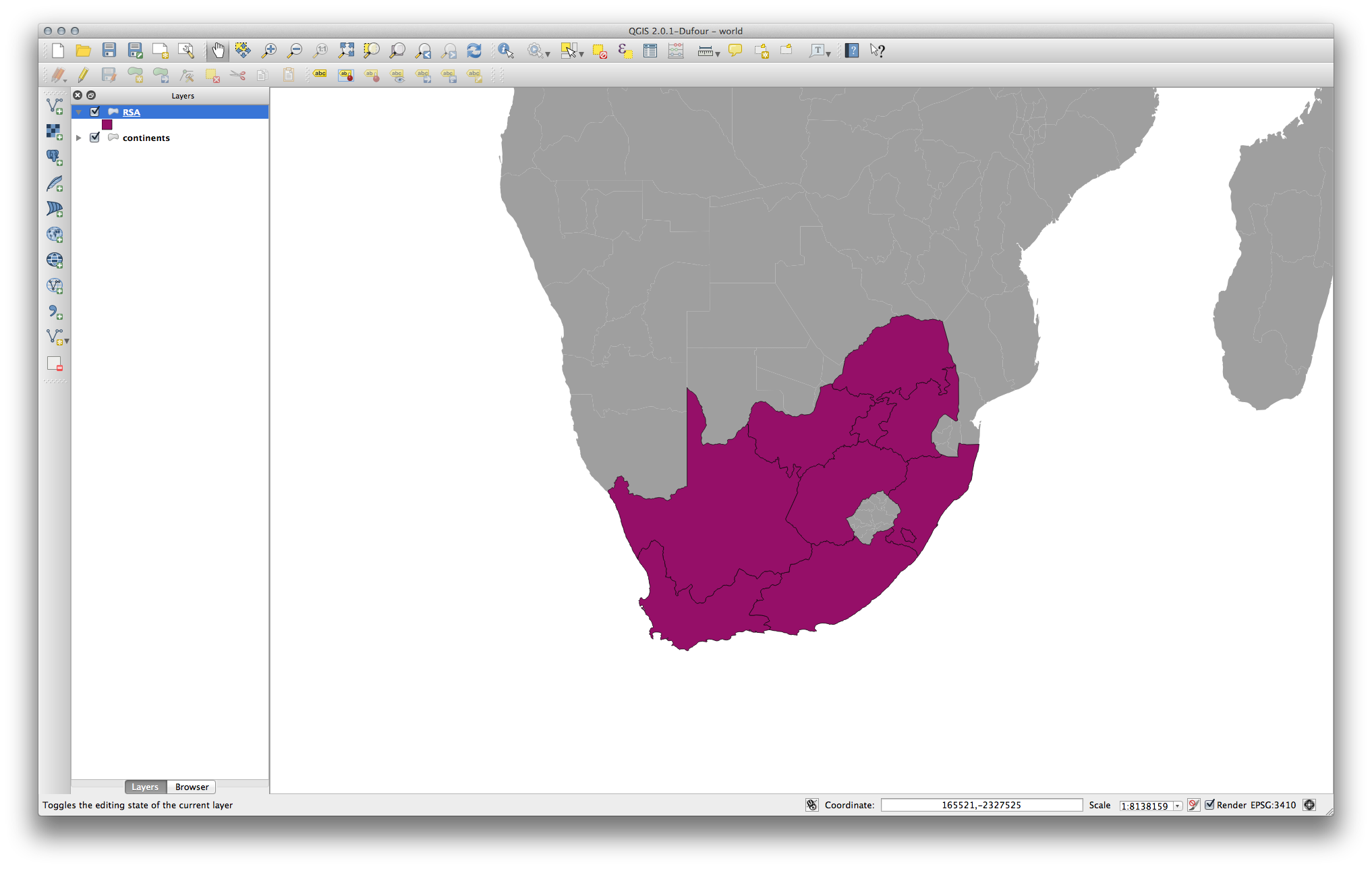
• Add another vector layer to your map which has the data for South Africa only. You’ll find it as exercise_data/world/RSA.shp.

何に気づくのですか？

レイヤは表示されません！しかし、修正するのは簡単ですよね？

• Right-click on the RSA layer in the Layers list.

• レイヤの領域にズーム を選択します。

そう、今は南アフリカが見えます・・・しかし世界の残りはどこですか？

It turns out that we can zoom between these two layers, but we can’t ever see them at the same time. That’s because their Coordinate Reference Systems are so different. The continents dataset is in degrees, but the RSA dataset is in meters. So, let’s say that a given point in Cape Town in the RSA dataset is about 4 100 000 meters away from the equator. But in the continents dataset, that same point is about 33.9 degrees away from the equator.

This is the same distance - but QGIS doesn’t know that. You haven’t told it to reproject the data. So as far as it’s concerned, the version of South Africa that we see in the RSA dataset has Cape Town at the correct distance of 4 100 000 meters from the equator. But in the continents dataset, Cape Town is only 33.9 meters away from the equator! You can see why this is a problem.

QGIS doesn’t know where Cape Town is supposed to be - that’s what the data should be telling it. If the data tells QGIS that Cape Town is 34 meters away from the equator and that South Africa is only about 12 meters from north to south, then that is what QGIS will draw.

これを正すには:

• Click on the CRS Status button again and switch Enable ‘on the fly’ CRS transformation on again as before.
• Zoom to the extents of the RSA dataset.

Now, because they’re made to project in the same CRS, the two datasets fit perfectly:

When combining data from different sources, it’s important to remember that they might not be in the same CRS. “On the fly” reprojection helps you to display them together.

Before you go on, you probably want to have the ‘on the fly’ reprojection to be automatically activated whenever you open datasets having different CRS:

• 再度 設定 ‣ オプション... を実行し、 CRS を選択します。

• もしレイヤが異なる座標系を持つ場合,自動で ‘オンザフライ’ リプロジェクションを有効にする をチェックします。

7.1.3. Follow Along: 他のCRSに設定したデータセットの保存¶

Remember when you calculated areas for the buildings in the Classification lesson? You did it so that you could classify the buildings according to area.

• あなたの通常のマップ（ Swellendam データを含む）を開きます。

• Open the attribute table for the buildings layer.

• :kbd:`AREA`フィールドが見えるまで右側にスクロールします。

Notice how the areas are all very small; probably zero. This is because these areas are given in degrees - the data isn’t in a Projected Coordinate System. In order to calculate the area for the farms in square meters, the data has to be in square meters as well. So, we’ll need to reproject it.

But it won’t help to just use ‘on the fly’ reprojection. ‘On the fly’ does what it says - it doesn’t change the data, it just reprojects the layers as they appear on the map. To truly reproject the data itself, you need to export it to a new file using a new projection.

• Right-click on the buildings layer in the Layers list.
• Select Save As... in the menu that appears. You will be shown the Save vector layer as... dialog.
• Click on the Browse button next to the Save as field.
• Navigate to exercise_data/ and specify the name of the new layer as buildings_reprojected.shp.

• エンコーディング はそのままにしておきます。

• Change the value of the Layer CRS dropdown to Selected CRS.

• ドロップダウン下の ブラウズ ボタンをクリックします。

• CRS セレクタ ダイアログが表示されるでしょう。

• :guilabel:`フィルター`フィールドで、 :kbd:`34S`を検索します。

• リストから :guilabel:`WGS 84 / UTM zone 34S`を選択します。

• Leave the Symbology export unchanged.

The Save vector layer as... dialog now looks like this:

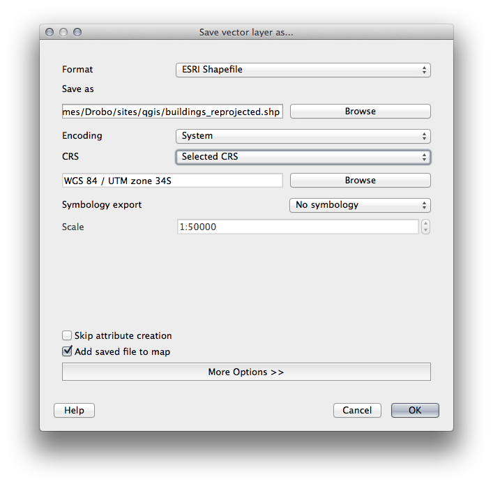
• Click OK.
• Start a new map and load the reprojected layer you just created.

Refer back to the lesson on Classification to remember how you calculated areas.

• Update (or add) the AREA field by running the same expression as before:

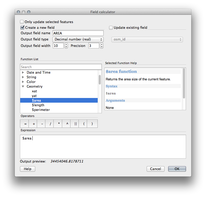
This will add an AREA field with the size of each building in square meters

• To calculate the area in another unit of measurement, for example hectares, use the AREA field to create a second column:

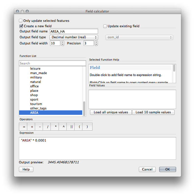
Look at the new values in your attribute table. This is much more useful, as people actually quote building size in meters, not in degrees. This is why it’s a good idea to reproject your data, if necessary, before calculating areas, distances, and other values that are dependent on the spatial properties of the layer.

7.1.4. Follow Along: 独自の投影法の作成¶

There are many more projections than just those included in QGIS by default. You can also create your own projections.

• マップを新規に開始します。

• Load the world/oceans.shp dataset.
• Go to Settings ‣ Custom CRS... and you’ll see this dialog:

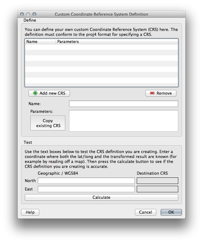
• Click on the Add new CRS button to create a new projection.

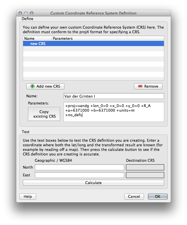
An interesting projection to use is called Van der Grinten I.

• 名称 フィールドでその名称を入力します。

This projection represents the Earth on a circular field instead of a rectangular one, as most other projections do.

• そのパラメータとして、次の文字列を使います：

+proj=vandg +lon_0=0 +x_0=0 +y_0=0 +R_A +a=6371000 +b=6371000 +units=m +no_defs

• Click OK.

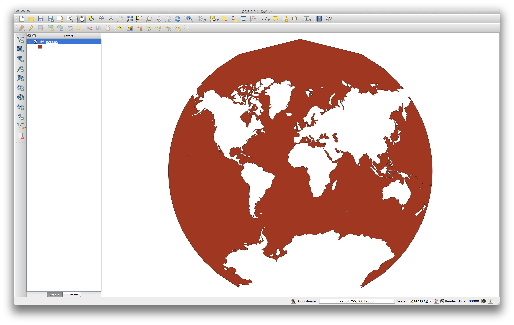
• “オンザフライ”再投影を有効にします。

• Choose your newly defined projection (search for its name in the Filter field).

• この投影法を適用するため、したがってマップは再投影されるでしょう：

7.1.5. In Conclusion¶

Different projections are useful for different purposes. By choosing the correct projection, you can ensure that the features on your map are being represented accurately.

7.1.6. Further Reading¶

Materials for the Advanced section of this lesson were taken from this article.

Further information on Coordinate Reference Systems is available here.

7.1.7. What’s Next?¶

次のレッスンでは、QGISの様々なベクタ分析ツールを使ってベクタデータの分析をする方法について学習します。