7.2. Lesson: ベクタ分析¶

7.2.1. GISプロセス¶

始める前に、任意のGISの問題を解決するために使用できるプロセスの簡単な概要を与えることが有用でしょう。それを行う方法は次のとおりです。

1. 問題の状態

2. データの入手

3. 問題の分析

4. 結果のプレゼン

7.2.2. 問題¶

Let’s start off the process by deciding on a problem to solve. For example, you are an estate agent and you are looking for a residential property in Swellendam for clients who have the following criteria:

1. Swellendam である必要がある。

2. 学校前の距離が、合理的にアクセスできる距離（例えば1km）である必要がある。

3. サイズが100m四方以上である必要がある。

4. 主要道路から50mより近い。

5. レストランから500m以内にある。

7.2.3. データ¶

これらの疑問に答えるため、次のデータが必要になるでしょう:

1. このエリアの住宅地属性(建物)。

2. 街とその周辺の道路

3. 学校とレストランの位置

4. 建物のサイズ

All of this data is available through OSM and you should find that the dataset you have been using throughout this manual can also be used for this lesson. However, in order to ensure we have the complete data, we will re-download the data from OSM using QGIS’ built-in OSM download tool.

7.2.4. Follow Along: プロジェクトの開始¶

• 新規のQGISプロジェクトの開始

• Use the OpenStreetMap data download tool found in the Vector -> OpenStreetMap menu to download the data for your chosen region.
• Save the data as osm_data.osm in your exercise_data folder.
• Note that the osm format is a type of vector data. Add this data as a vector layer as usually Layer -> Add vector layer..., browse to the new osm_data.osm file you just downloaded. You may need to select Show All Files as the file format.

• osm_data.osm を選択し 開く をクリックします。

• 表示されたダイアログで、 except the other_relations と multilinestrings layer: のすべてのレイヤを選択します。

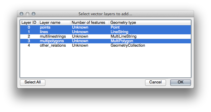
これで、あなたのマップに分断されたレイヤとしてOSMデータをインポートできます。

The data you just downloaded from OSM is in a geographic coordinate system, WGS84, which uses latitude and longitude coordinates, as you know from the previous lesson. You also learnt that to calculate distances in meters, we need to work with a projected coordinate system. Start by setting your project’s coordinate system to a suitable CRS for your data, in the case of Swellendam, WGS 84 / UTM zone 34S:

• Open the Project Properties dialog, select CRS and filter the list to find WGS 84 / UTM zone 34S.
• Click OK.

We now need to extract the information we need from the OSM dataset. We need to end up with layers representing all the houses, schools, restaurants and roads in the region. That information is inside the multipolygons layer and can be extracted using the information in its Attribute Table. We’ll start with the schools layer:

• Right-click on the multipolygons layer in the Layers list and open the Layer Properties.

• 一般情報 メニューに進みます。

• Under Feature subset click on the [Query Builder] button to open the Query builder dialog.
• In the Fields list on the left of this dialog until you see the field amenity.

• それを１回だけクリックします。

• :guilabel:`値`リストで:guilabel:`すべて`ボタンをクリックします:

さて我々はQGISに:kbd:amenity が :kbd:`school`に等しいポリゴンであることのみ示す必要があります。

• フィールド リストの amenity をダブルクリックします。

• Watch what happens in the Provider specific filter expression field below:

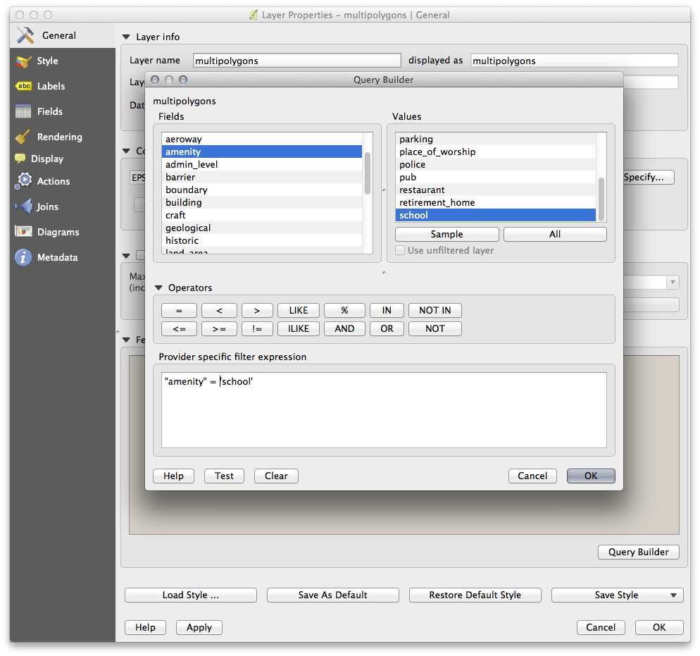
The word "amenity" has appeared. To build the rest of the query:

• （:guilabel:`演算子`から） :guilabel:`=`ボタンをクリックします。

• 値 リストで school の値をダブルクリックします。

• OK を２回クリックします。

This will filter OSM’s multipolygons layer to only show the schools in your region. You can now either:

• Rename the filtered OSM layer to schools and re-import the multipolygons layer from osm_data.osm, OR
• Duplicate the filtered layer, rename the copy, clear the Query Builder and create your new query in the Query Builder.

7.2.5. |TY|OSMからの必要なレイヤの抽出¶

Using the above technique, use the Query Builder tool to extract the remaining data from OSM to create the following layers:

• roads (OSMの lines レイヤ由来)

• restaurants (OSMの multipolygons レイヤ由来)

• houses (OSMの multipolygons レイヤ由来)

前のレッスンで作成した roads.shp を再利用するのが望ましいです。

結果の確認

• Save your map under exercise_data, as analysis.qgs (this map will be used in future modules).
• In your operating system’s file manager, create a new folder under exercise_data and call it residential_development. This is where you’ll save the datasets that will be the results of the analysis functions.

7.2.6. Try Yourself 主要道路の検索¶

Some of the roads in OSM’s dataset are listed as unclassified, tracks, path and footway. We want to exclude these from our roads dataset.

• Open the Query Builder for the roads layer, click Clear and build the following query:

  "highway"  != 'NULL' AND "highway" != 'unclassified' AND "highway" != 'track' AND "highway" != 'path' AND "highway" != 'footway'

You can either use the approach above, where you double-clicked values and clicked buttons, or you can copy and paste the command above.

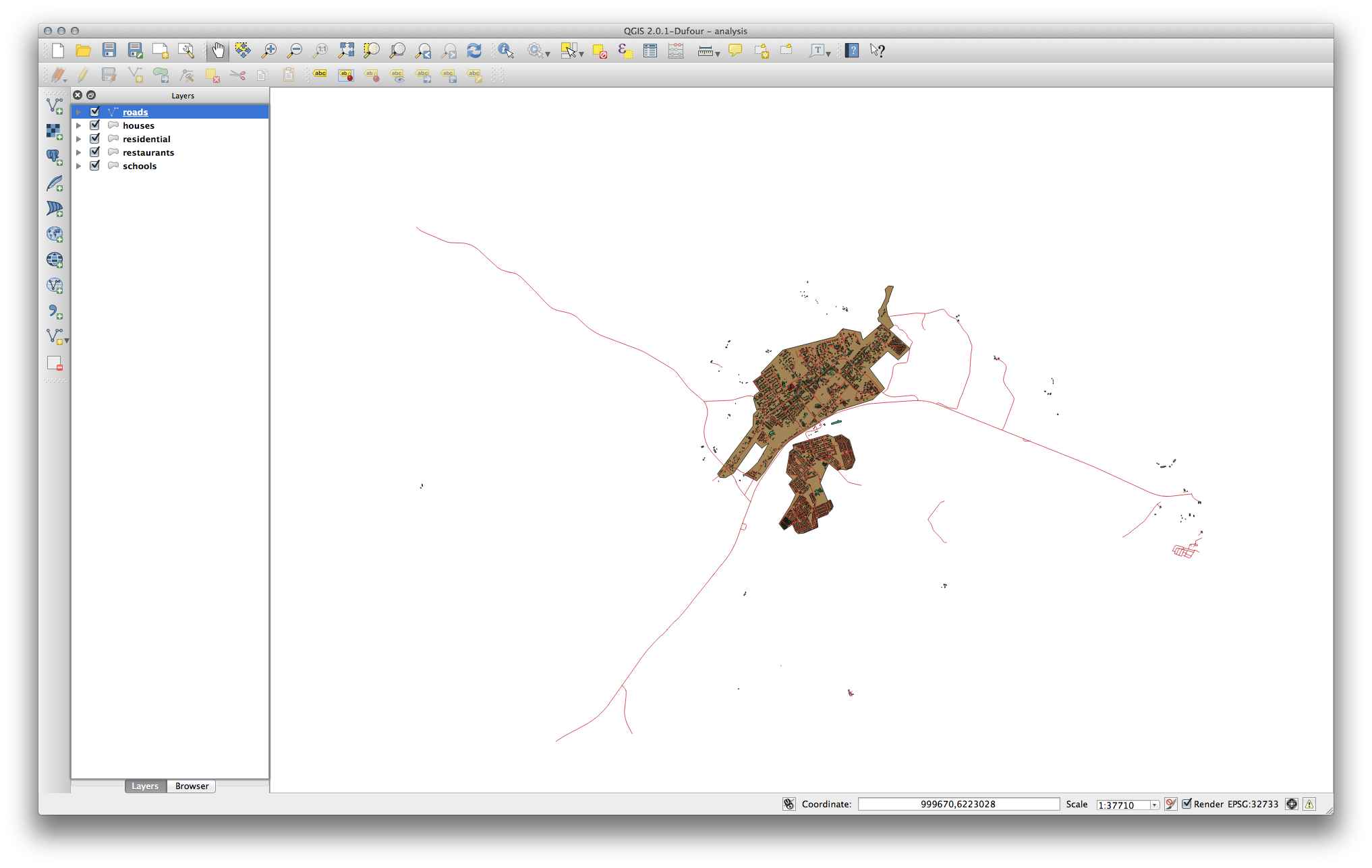
直ちにマップから多くの道路を減らすべきです:

7.2.7. Try Yourself レイヤCRSの変換¶

Because we are going to be measuring distances within our layers, we need to change the layers’ CRS. To do this, we need to select each layer in turn, save the layer to a new shapefile with our new projection, then import that new layer into our map.

• Right click the roads layer in the Layers panel.

• Save as... をクリックします。

• In the Save Vector As dialog, choose the following settings and click Ok (making sure you select Add saved file to map):

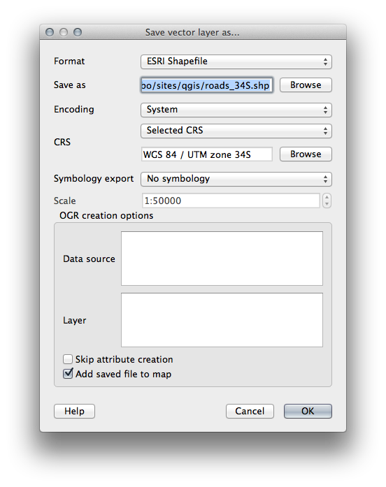
新しいシェープファイルが作成され、あなたのマップに結果のレイヤとして追加されます。

• 古い roads レイヤを削除します。

Repeat this process for each layer, creating a new shapefile and layer with “_34S” appended to the original name and removing each of the old layers.

Once you have completed the process for each layer, right click on any layer and click Zoom to layer extent to focus the map to the area of interest.

Now that we have converted OSM’s data to a UTM projection, we can begin our calculations.

7.2.8. Follow Along: 問題の分析:学校と道路からの距離¶

QGISはいかなるベクタからの距離を計算することができます。

• Make sure that only the roads_34S and houses_34S layers are visible, to simplify the map while you’re working.
• Click on the Vector ‣ Geoprocessing Tools ‣ Buffer(s) tool:

新しいダイアログを表示します。

• このように設定します:

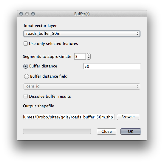
The Buffer distance is in meters because our input dataset is in a Projected Coordinate System that uses meter as its basic measurement unit. This is why we needed to use projected data.

• Save the resulting layer under exercise_data/residential_development/ as roads_buffer_50m.shp.

• OK をクリックし、バッファを作成します。

• When it asks you if it should “add the new layer to the TOC”, click Yes. (“TOC” stands for “Table of Contents”, by which it means the Layers list).
• Close the Buffer(s) dialog.

今すぐあなたのマップは次のようになります:

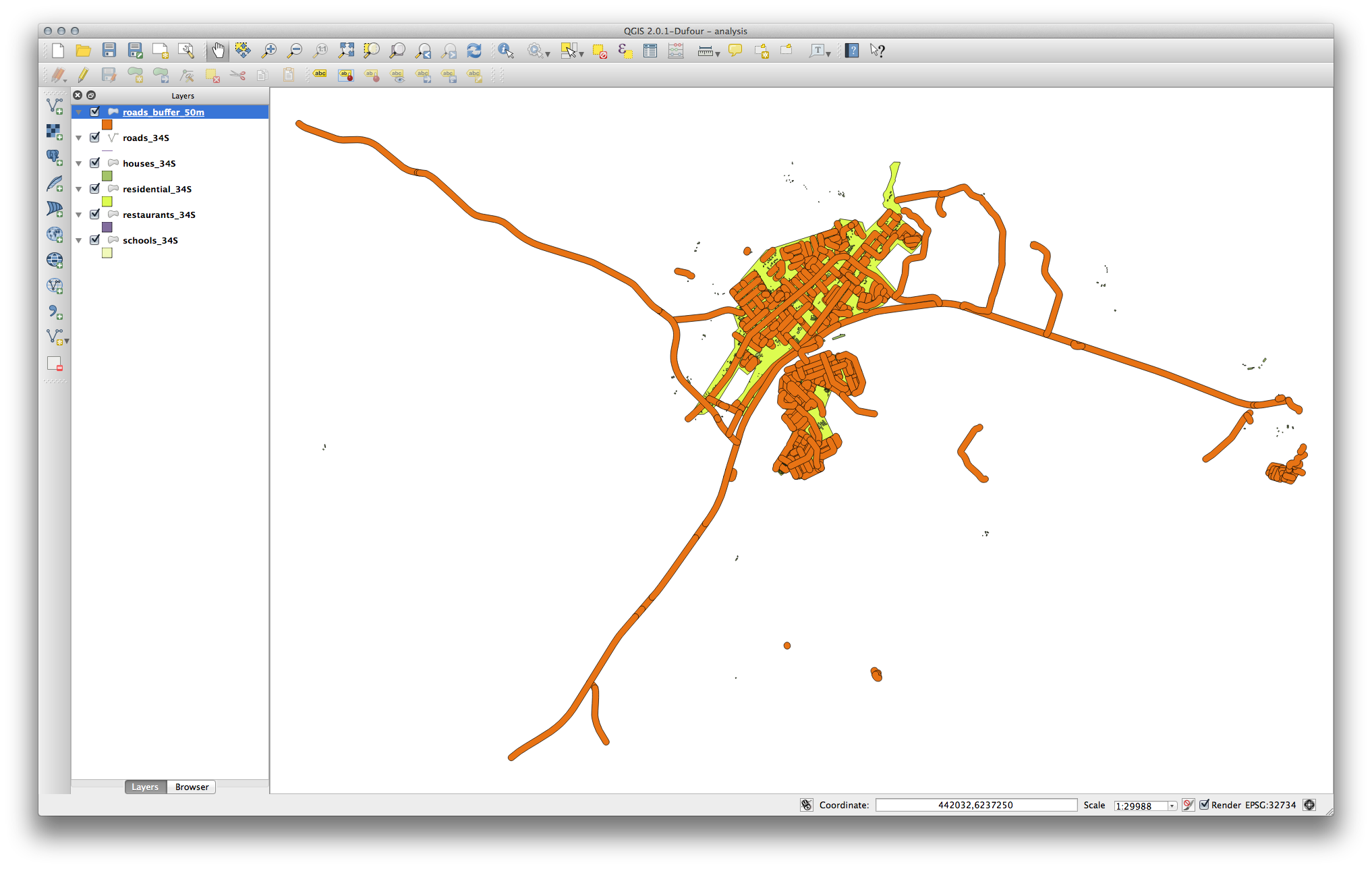
If your new layer is at the top of the Layers list, it will probably obscure much of your map, but this gives us all the areas in your region which are within 50m of a road.

However, you’ll notice that there are distinct areas within our buffer, which correspond to all the individual roads. To get rid of this problem, remove the layer and re-create the buffer using the settings shown here:

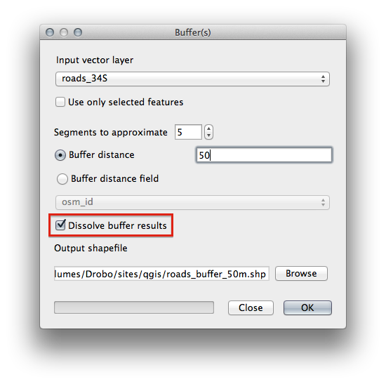
• バッファのディゾルブ結果 ボックスを今チェックしていることに注目ください。

• Save the output under the same name as before (click Yes when it asks your permission to overwrite the old one).

• OK をクリックし バッファ ダイアログを再度閉じます。

レイヤリスト にいったんレイヤを追加すると、このように見えます:

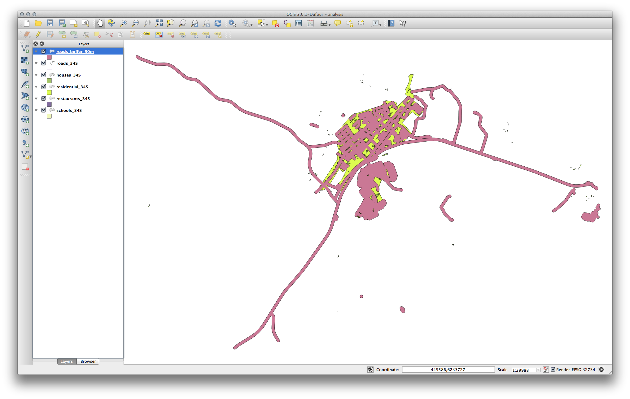
今不要な下位区分はありません。

7.2.9. Try Yourself 学校からの距離¶

• Use the same approach as above and create a buffer for your schools.

It needs to be 1 km in radius, and saved under the usual directory as schools_buffer_1km.shp.

結果の確認

7.2.10. Follow Along: 重複エリア¶

Now we have areas where the road is 50 meters away and there’s a school within 1 km (direct line, not by road). But obviously, we only want the areas where both of these criteria are satisfied. To do that, we’ll need to use the Intersect tool. Find it under Vector ‣ Geoprocessing Tools ‣ Intersect. Set it up like this:

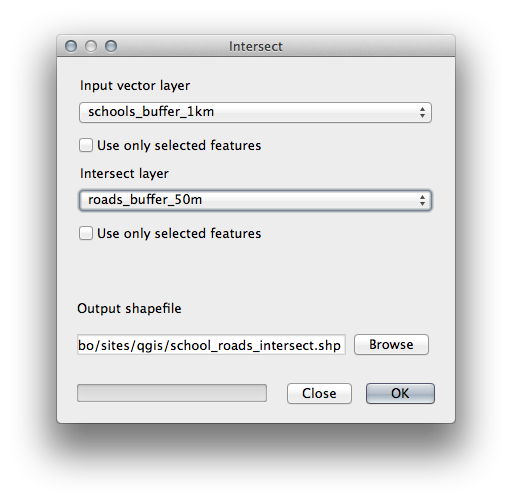
The two input layers are the two buffers; the save location is as usual; and the file name is road_school_buffers_intersect.shp. Once it’s set up like this, click OK and add the layer to the Layers list when prompted.

In the image below, the blue areas show us where both distance criteria are satisfied at once!

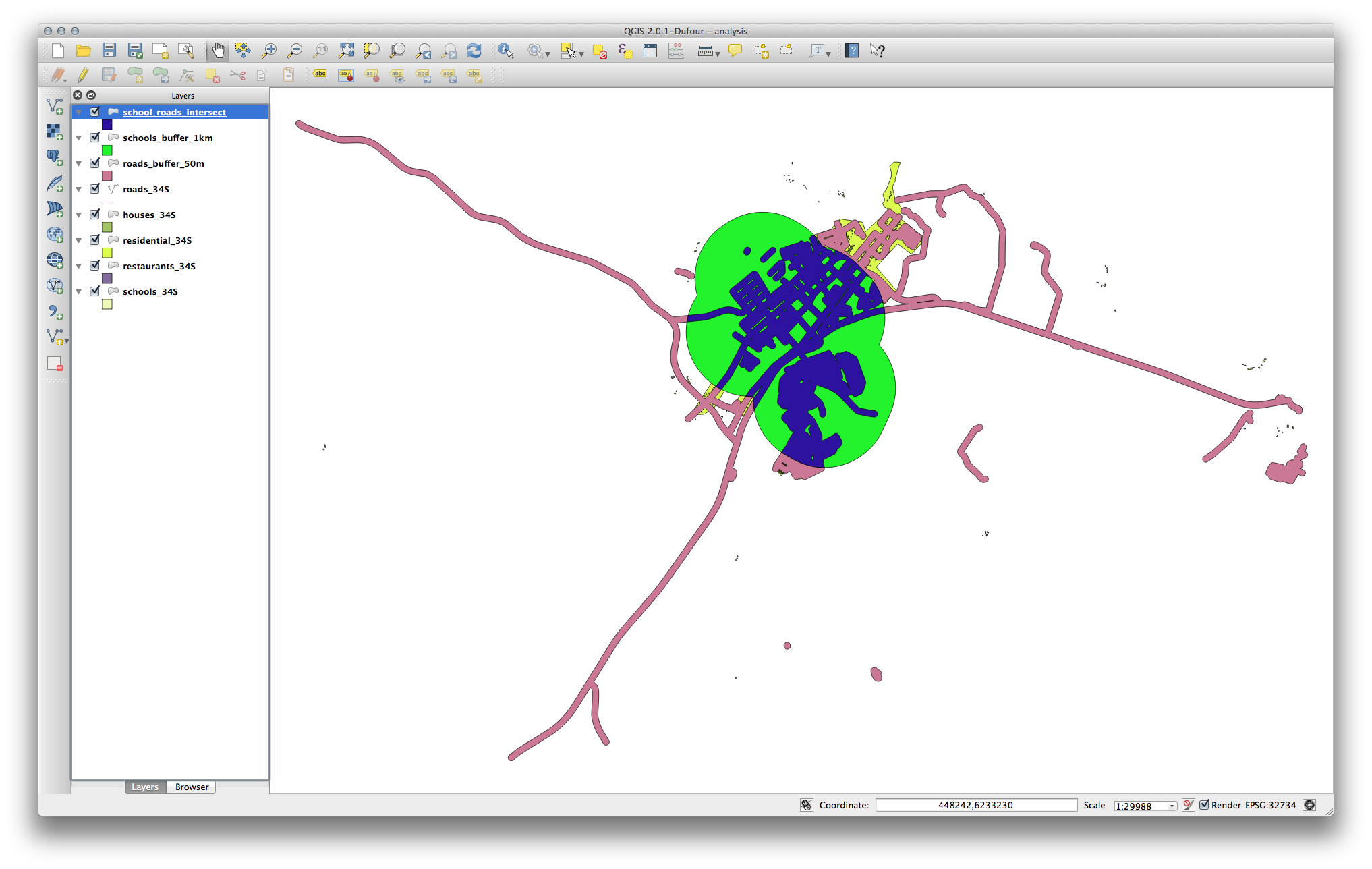
You may remove the two buffer layers and only keep the one that shows where they overlap, since that’s what we really wanted to know in the first place:

7.2.11. Follow Along: 建物の選択¶

Now you’ve got the area that the buildings must overlap. Next, you want to select the buildings in that area.

• Click on the menu entry Vector ‣ Research Tools ‣ Select by location. A dialog will appear.

• このように設定します:

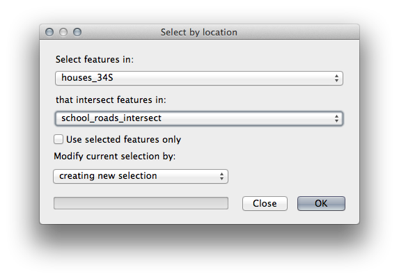
• OK をクリックし、 閉じる をクリックします。

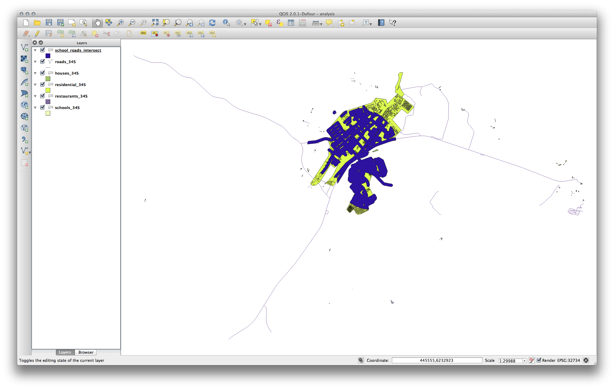
• You’ll probably find that not much seems to have changed. If so, move the school_roads_intersect layer to the bottom of the layers list, then zoom in:

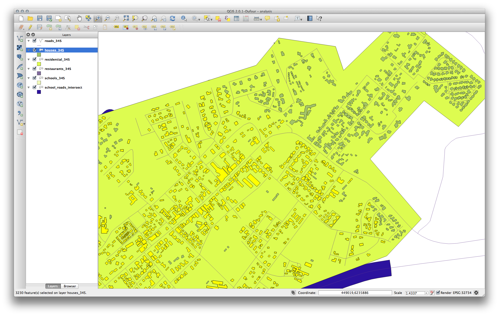
The buildings highlighted in yellow are those which match our criteria and are selected, while the buildings in green are those which do not. We can now save the selected buildings as a new layer.

• Right-click on the houses_34S layer in the Layers list.
• Select Save Selection As....

• ダイアログにてこのように設定します:

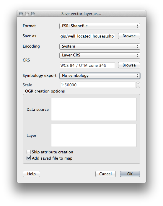
• ファイル名は well_located_houses.shp です。

• Click OK.

Now you have the selection as a separate layer and can remove the houses_34S layer.

7.2.12. Try Yourself Further Filter our Buildings¶

We now have a layer which shows us all the buildings within 1km of a school and within 50m of a road. We now need to reduce that selection to only show buildings which are within 500m of a restaurant.

Using the processes described above, create a new layer called houses_restaurants_500m which further filters your well_located_houses layer to show only those which are within 500m of a restaurant.

結果の確認

7.2.13. Follow Along: 正しいサイズの建物の選択¶

To see which buildings are the correct size (more than 100 square meters), we first need to calculate their size.

• Open the attribute table for the houses_restaurants_500m layer.

• 編集モードにし、フィールド演算を開きます。

• このように設定します:

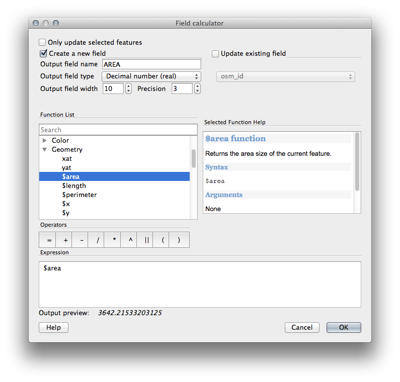
• If you can’t find AREA in the list, try creating a new field as you did in the previous lesson of this module.
• Click OK.
• Scroll to the right of the attribute table; your AREA field now has areas in metres for all the buildings in your houses_restaurants_500m layer.
• Click the edit mode button again to finish editing, and save your edits when prompted.
• Build a query as earlier in this lesson:

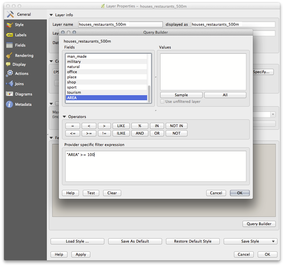
• Click OK. Your map should now only show you those buildings which match our starting criteria and which are more than 100m squared in size.

7.2.14. Try Yourself¶

• Save your solution as a new layer, using the approach you learned above for doing so. The file should be saved under the usual directory, with the name solution.shp.

7.2.15. In Conclusion¶

Using the GIS problem-solving approach together with QGIS vector analysis tools, you were able to solve a problem with multiple criteria quickly and easily.

7.2.16. What’s Next?¶

In the next lesson, we’ll look at how to calculate the shortest distance along the road from one point to another.