GRASS GIS の統合¶

GRASSプラグインの起動¶

QGISでGRASS の機能を利用したりGRASS ベクタとラスタレイヤを表示するためには, プラグインマネージャのGRASSプラグインを選択する必要があります. メニュー Plugins ‣ Manage Plugins, でselect GRASS を選び [OK]　をクリックして下さい.

ここで 既存の GRASS LOCATION ( セクション GRASSラスタとベクタレイヤのロード 参照 ) からラスタとベクタレイヤをロードできます. また新しい GRASS LOCATION を QGIS で (セクション 新しいGRASS LOCATIONの作成 参照) 作成したりいくつかのラスタやベクタデータを (セクション GRASS LOCATIONへデータをインポート 参照) GRASS ツールボックス (セクション GRASSツールボックス 参照) のすばらしい解析機能で使うためにインポートすることができます.

GRASSラスタとベクタレイヤのロード¶

GRASS プラグインで,ツールバーメニューの上の適切なボタンをクリックしてベクタやラスタのレイヤをロードすることができます. 例として QGIS アラスカデータセット (セクション サンプルデータ 参照) を使えます. ここには小さめの GRASSサンプルとして LOCATION として3 個のベクタレイヤと1個のラスタ標高マップがあります.

1. Create a new folder called grassdata, download the QGIS ‘Alaska’ dataset qgis_sample_data.zip from http://download.osgeo.org/qgis/data/ and unzip the file into grassdata.

2. QGIS を開始してください

3. もし事前の QGIS セッションで,GRASS プラグインをロードしていない場合は Plugins ‣ Manage Plugins をクリックして GRASS を有効にして下さい. GRASS ツールバーが QGIS メインウィンドウに表示されます.

4. GRASS ツールバーで ^{Open mapset} アイコンをクリックすると MAPSET ウィザードが起動します.

5. For Gisdbase, browse and select or enter the path to the newly created folder grassdata.
6. You should now be able to select the LOCATION alaska and the MAPSET demo.
7. Click [OK]. Notice that some previously disabled tools in the GRASS toolbar are now enabled.
8. Click on ^{Add GRASS raster layer}, choose the map name gtopo30 and click [OK]. The elevation layer will be visualized.
9. Click on ^{Add GRASS vector layer}, choose the map name alaska and click [OK]. The Alaska boundary vector layer will be overlayed on top of the gtopo30 map. You can now adapt the layer properties as described in chapter ベクタプロパティダイアログ (e.g., change opacity, fill and outline color).

10. その他の2つのベクタレイヤ rivers and airports をロードしてプロパティを調整して下さい.

ご覧になったようにGRASSのラスタとベクタレイヤをQGISにロードする方法はとても簡単です. 以下のセクションではGRASS データの編集と新しい LOCATION の作成について記述されています . さらに多くのサンプル GRASS LOCATIONs が GRASS ウェッブサイト http://grass.osgeo.org/download/sample-data/ にあります.

GRASS LOCATIONとMAPSET¶

GRASS data are stored in a directory referred to as GISDBASE. This directory, often called grassdata, must be created before you start working with the GRASS plugin in QGIS. Within this directory, the GRASS GIS data are organized by projects stored in subdirectories called LOCATIONs. Each LOCATION is defined by its coordinate system, map projection and geographical boundaries. Each LOCATION can have several MAPSETs (subdirectories of the LOCATION) that are used to subdivide the project into different topics or subregions, or as workspaces for individual team members (see Neteler & Mitasova 2008 in 文献とWeb参照). In order to analyze vector and raster layers with GRASS modules, you must import them into a GRASS LOCATION. (This is not strictly true – with the GRASS modules r.external and v.external you can create read-only links to external GDAL/OGR-supported datasets without importing them. But because this is not the usual way for beginners to work with GRASS, this functionality will not be described here.)

Figure GRASS location 1:

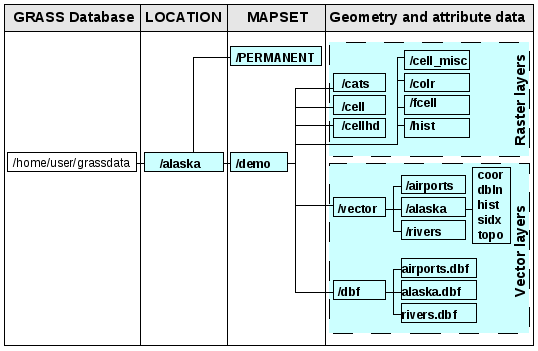
alaska LOCATIONのGRASSデータ

新しいGRASS LOCATIONの作成¶

ここに例として用意した GRASS LOCATION alaska, は Albers正積投影でフィート単位で作成されているプロジェクトの QGISサンプルデータセットです. このサンプルThis sample GRASS LOCATION alaska は次のGRASS GIS 関連の章で例と演習に使われます.これはダウンロードしてあなたのコンピュータにインストールできる便利なデータセットです(ref:label_sampledata 参照).

1. QGIS を起動して GRASS プラグインがロードされているかどうか確認して下さい.

2. QGIS のアラスカデータセット サンプルデータ から alaska.shp shapefile (セクション vector_load_shapefile 参照) を表示します (セクション vector_load_shapefile 参照) .

3. GRASS ツールバーで ^{New mapset} アイコンをクリックして MAPSET ウィザードを起動して下さい.

4. 既存の GRASS データベース (GISDBASE) フォルダ grassdata を選択するかあなたのコンピュータのファイルマネージャを使って新しい LOCATION を作成して下さい. それから [Next] をクリックして下さい.

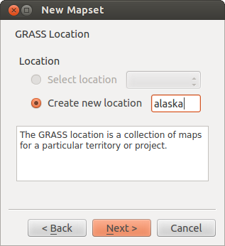
5. We can use this wizard to create a new MAPSET within an existing LOCATION (see section 新しいMAPSETの追加) or to create a new LOCATION altogether. Select Create new location (see figure_grass_location_2).
6. Enter a name for the LOCATION – we used ‘alaska’ – and click [Next].
7. Define the projection by clicking on the radio button Projection to enable the projection list.
8. We are using Albers Equal Area Alaska (feet) projection. Since we happen to know that it is represented by the EPSG ID 2964, we enter it in the search box. (Note: If you want to repeat this process for another LOCATION and projection and haven’t memorized the EPSG ID, click on the ^{CRS Status} icon in the lower right-hand corner of the status bar (see section 投影法の利用方法)).
9. In Filter, insert 2964 to select the projection.

10. [次へ] をクリックして下さい.

11. To define the default region, we have to enter the LOCATION bounds in the north, south, east, and west directions. Here, we simply click on the button [Set current |qg| extent], to apply the extent of the loaded layer alaska.shp as the GRASS default region extent.

12. [次へ] をクリックして下さい.

13. We also need to define a MAPSET within our new LOCATION (this is necessary when creating a new LOCATION). You can name it whatever you like - we used ‘demo’. GRASS automatically creates a special MAPSET called PERMANENT, designed to store the core data for the project, its default spatial extent and coordinate system definitions (see Neteler & Mitasova 2008 in 文献とWeb参照).
14. Check out the summary to make sure it’s correct and click [Finish].

15. 新しい LOCATION ‘alaska’ と２つの MAPSETs ‘demo’ と ‘PERMANENT’ が作られました. 現在オープンされているワーキングセットはあなたが定義した ‘demo’ です.

16. GRASSツールバーのそれまでは利用できなかったいくつかのツールが利用可能になっています.

Figure GRASS location 2:

Creating a new GRASS LOCATION or a new MAPSET in QGIS

If that seemed like a lot of steps, it’s really not all that bad and a very quick way to create a LOCATION. The LOCATION ‘alaska’ is now ready for data import (see section GRASS LOCATIONへデータをインポート). You can also use the already-existing vector and raster data in the sample GRASS LOCATION ‘alaska’, included in the QGIS ‘Alaska’ dataset サンプルデータ, and move on to section GRASSベクターデータモデル.

GRASS LOCATIONへデータをインポート¶

This section gives an example of how to import raster and vector data into the ‘alaska’ GRASS LOCATION provided by the QGIS ‘Alaska’ dataset. Therefore, we use the landcover raster map landcover.img and the vector GML file lakes.gml from the QGIS ‘Alaska’ dataset (see サンプルデータ).

1. QGIS を起動して GRASS プラグインがロードされているかどうか確認して下さい.

2. GRASS ツールバーで ^{Open MAPSET} アイコンをクリックして MAPSET ウィザードを起動して下さい.

3. QGIS アラスカデータセットの中の grassdata フォルダーをGRASSデータベースとして選択して下さい, LOCATION を ‘alaska’ , MAPSET 　を ‘demo’ として [OK] をクリックして下さい.

4. ここで ^{Open GRASS tools} アイコンをクリックして下さい. GRASS ツールボックス (セクション subsec_grass_toolbox 参照) ダイアログが表示されます.

5. ラスタマップ landcover.img をインポートする場合 Modules Tree タブの r.in.gdal モジュールをクリックして下さい. この GRASSモジュールは GDAL がサポートしているファイルをGRASS LOCATION にインポートします. r.in.gdal モジュールダイアログが表示されます.

6. Browse to the folder raster in the QGIS ‘Alaska’ dataset and select the file landcover.img.

7. ラスタの出力名称として landcover_grass を指定して [Run] をクリックして下さい. Output タブには実行しているGRASS コマンド r.in.gdal -o input=/path/to/landcover.img output=landcover_grass が表示されます.

8. When it says Succesfully finished, click [View output]. The landcover_grass raster layer is now imported into GRASS and will be visualized in the QGIS canvas.
9. To import the vector GML file lakes.gml, click the module v.in.ogr in the Modules Tree tab. This GRASS module allows you to import OGR-supported vector files into a GRASS LOCATION. The module dialog for v.in.ogr appears.
10. Browse to the folder gml in the QGIS ‘Alaska’ dataset and select the file lakes.gml as OGR file.
11. As vector output name, define lakes_grass and click [Run]. You don’t have to care about the other options in this example. In the Output tab you see the currently running GRASS command v.in.ogr -o dsn=/path/to/lakes.gml output=lakes\_grass.
12. When it says Succesfully finished, click [View output]. The lakes_grass vector layer is now imported into GRASS and will be visualized in the QGIS canvas.

GRASSベクターデータモデル¶

デジタイズの前に GRASSベクターデータモデル を理解することは重要です.

基本的にGRASSではトポロジカルベクターモデルを使用します.

This means that areas are not represented as closed polygons, but by one or more boundaries. A boundary between two adjacent areas is digitized only once, and it is shared by both areas. Boundaries must be connected and closed without gaps. An area is identified (and labeled) by the centroid of the area.

Besides boundaries and centroids, a vector map can also contain points and lines. All these geometry elements can be mixed in one vector and will be represented in different so-called ‘layers’ inside one GRASS vector map. So in GRASS, a layer is not a vector or raster map but a level inside a vector layer. This is important to distinguish carefully. (Although it is possible to mix geometry elements, it is unusual and, even in GRASS, only used in special cases such as vector network analysis. Normally, you should prefer to store different geometry elements in different layers.)

It is possible to store several ‘layers’ in one vector dataset. For example, fields, forests and lakes can be stored in one vector. An adjacent forest and lake can share the same boundary, but they have separate attribute tables. It is also possible to attach attributes to boundaries. An example might be the case where the boundary between a lake and a forest is a road, so it can have a different attribute table.

The ‘layer’ of the feature is defined by the ‘layer’ inside GRASS. ‘Layer’ is the number which defines if there is more than one layer inside the dataset (e.g., if the geometry is forest or lake). For now, it can be only a number. In the future, GRASS will also support names as fields in the user interface.

Attributes can be stored inside the GRASS LOCATION as dBase or SQLite3 or in external database tables, for example, PostgreSQL, MySQL, Oracle, etc.

データベーステーブルの属性とリンクされたジオメトリエレメントを ‘カテゴリ’ 値として使ってます.

‘Category’ (key, ID) is an integer attached to geometry primitives, and it is used as the link to one key column in the database table.

新しいGRASSベクターレイヤーの作成¶

To create a new GRASS vector layer with the GRASS plugin, click the ^{Create new GRASS vector} toolbar icon. Enter a name in the text box, and you can start digitizing point, line or polygon geometries following the procedure described in section GRASSベクタレイヤのデジタイジングと編集.

In GRASS, it is possible to organize all sorts of geometry types (point, line and area) in one layer, because GRASS uses a topological vector model, so you don’t need to select the geometry type when creating a new GRASS vector. This is different from shapefile creation with QGIS, because shapefiles use the Simple Feature vector model (see section 新しいベクタレイヤの作成).

GRASSベクタレイヤのデジタイジングと編集¶

The digitizing tools for GRASS vector layers are accessed using the ^{Edit GRASS vector layer} icon on the toolbar. Make sure you have loaded a GRASS vector and it is the selected layer in the legend before clicking on the edit tool. Figure figure_grass_digitizing_2 shows the GRASS edit dialog that is displayed when you click on the edit tool. The tools and settings are discussed in the following sections.

ツールバー

In figure_grass_digitizing_1, you see the GRASS digitizing toolbar icons provided by the GRASS plugin. Table table_grass_digitizing_1 explains the available functionalities.

Figure GRASS digitizing 1:

GRASSデジタイズツールバー

アイコン	ツール	目的
	新しい点	新しい点をデジタイズ
	新しいライン	新しいラインをデジタイズ
	新しい境界	新しい境界をデジタイズ (その他のツールを選択することで終了します)
	セントロイドの新規作成	新しいセントロイドをデジタイズ (ラベルのあるエリア)
	端点の移動	ライン上の端点を特定して移動する
	端点の追加	ラインに新たな端点の追加
	端点の除去	ライン上の端点を削除する (2回クリックすることで選択)
	要素の移動	クリックして選択した境界, ライン, 点, セントロイドを移動
	ラインの切断	ラインを2つに切断
	要素の削除	境界, ライン, 点, セントロイドの削除 (2回クリックすることで選択)
	属性の編集	選択した要素の属性を編集 (上のように, 1つの要素に対して1つ以上のフィーチャを表現できます)
	閉じる	セッションを閉じて現在のステータスを保存して下さい (しばらくするとトポロジーがリビルドされます)

表 GRASS デジタイジング 1: GRASS デジタイジングツール

カテゴリータブ

The Category tab allows you to define the way in which the category values will be assigned to a new geometry element.

Figure GRASS digitizing 2:

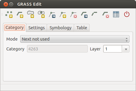
GRASSデジタイズカテゴリータブ

• モード: どのカテゴリ値が新しいジオメトリエレメントに割り当てられるか.

  • 次に使っていないもの - 次に使っていないカテゴリ値をジオメトリエレメントに割り当てます.

  • 手動エントリ - ジオメトリエレメントに割り当てる値を ‘カテゴリ’-エントリフィールドで手動で定義します.

  • カテゴリ無し - ジオメトリエレメントにカテゴリ値を割り当てない. たとえばエリアの境界線,この場合カテゴリ値はセントロイドに結び付けられます.

• カテゴリ - それぞれのデジタイズされたジオメトリエレメントに割り当てられた数値 (ID) . それぞれのジオメトリエレメントと属性を結合します.

• フィールド (レイヤ) - それぞれのジオメトリエレメントは異なるGRASSジオメトリレイヤを使って様々な属性テーブルに結合できます. デフォルトレイヤ番号は1です.

選択タブ

The Settings tab allows you to set the snapping in screen pixels. The threshold defines at what distance new points or line ends are snapped to existing nodes. This helps to prevent gaps or dangles between boundaries. The default is set to 10 pixels.

Figure GRASS digitizing 3:

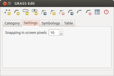
GRASSデジタイズ設定タブ

シンボルタブ

The Symbology tab allows you to view and set symbology and color settings for various geometry types and their topological status (e.g., closed / opened boundary).

Figure GRASS digitizing 4:

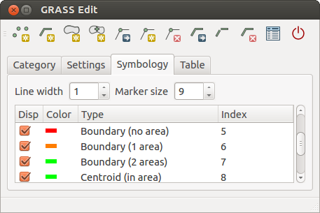
GRASSデジタイズシンボロジータブ

テーブルタブ

The Table tab provides information about the database table for a given ‘layer’. Here, you can add new columns to an existing attribute table, or create a new database table for a new GRASS vector layer (see section 新しいGRASSベクターレイヤーの作成).

Figure GRASS digitizing 5:

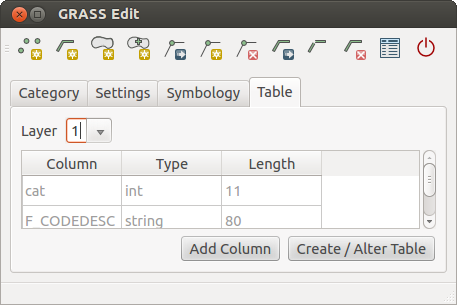
GRASSテーブル編集タブ

GRASS領域ツール¶

The region definition (setting a spatial working window) in GRASS is important for working with raster layers. Vector analysis is by default not limited to any defined region definitions. But all newly created rasters will have the spatial extension and resolution of the currently defined GRASS region, regardless of their original extension and resolution. The current GRASS region is stored in the $LOCATION/$MAPSET/WIND file, and it defines north, south, east and west bounds, number of columns and rows, horizontal and vertical spatial resolution.

It is possible to switch on and off the visualization of the GRASS region in the QGIS canvas using the ^{Display current GRASS region} button.

With the ^{Edit current GRASS region} icon, you can open a dialog to change the current region and the symbology of the GRASS region rectangle in the QGIS canvas. Type in the new region bounds and resolution, and click [OK]. The dialog also allows you to select a new region interactively with your mouse on the QGIS canvas. Therefore, click with the left mouse button in the QGIS canvas, open a rectangle, close it using the left mouse button again and click [OK].

The GRASS module g.region provides a lot more parameters to define an appropriate region extent and resolution for your raster analysis. You can use these parameters with the GRASS Toolbox, described in section GRASSツールボックス.

GRASSツールボックス¶

The ^{Open GRASS Tools} box provides GRASS module functionalities to work with data inside a selected GRASS LOCATION and MAPSET. To use the GRASS Toolbox you need to open a LOCATION and MAPSET that you have write permission for (usually granted, if you created the MAPSET). This is necessary, because new raster or vector layers created during analysis need to be written to the currently selected LOCATION and MAPSET.

Figure GRASS Toolbox 1:

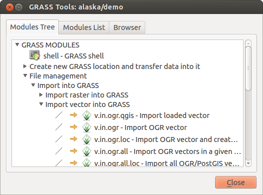
GRASSツールボックスとモジュールツリー

GRASSモジュールを使用します¶

The GRASS shell inside the GRASS Toolbox provides access to almost all (more than 300) GRASS modules in a command line interface. To offer a more user-friendly working environment, about 200 of the available GRASS modules and functionalities are also provided by graphical dialogs within the GRASS plugin Toolbox.

QGIS バージョン 2.6 のグラフィカルツールボックスで利用可能なGRASSモジュールの完全なリストはGRASS wiki http://grass.osgeo.org/wiki/GRASS-QGIS_relevant_module_list に記述されています.

GRASS ツールボックスの内容をカスタマイズできます. この機能は セクション GRASSツールボックスのカスタマイズ に記述されています.

As shown in figure_grass_toolbox_1, you can look for the appropriate GRASS module using the thematically grouped Modules Tree or the searchable Modules List tab.

By clicking on a graphical module icon, a new tab will be added to the Toolbox dialog, providing three new sub-tabs: Options, Output and Manual.

オプション

The Options tab provides a simplified module dialog where you can usually select a raster or vector layer visualized in the QGIS canvas and enter further module-specific parameters to run the module.

Figure GRASS module 1:

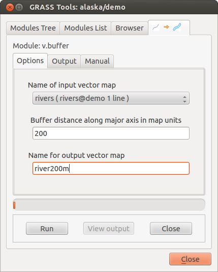
GRASSツールボックスモジュールオプション

The provided module parameters are often not complete to keep the dialog clear. If you want to use further module parameters and flags, you need to start the GRASS shell and run the module in the command line.

QGIS 1.8 からの新しい機能として Options タブの簡素化ダイアログの下の show advanced options ボタンがあります. 現状で v.in.ascii　モジュールの例としての使用が追加されているだけですが, しかし将来のバージョンのQGISでは GRASSツールボックスにさらに多くの機能が追加されるでしょう. このことによってGRASSの完全なモジュールがGRASSシェルに切り替えしなくても利用できるようになるでしょう.

出力

Figure GRASS module 2:

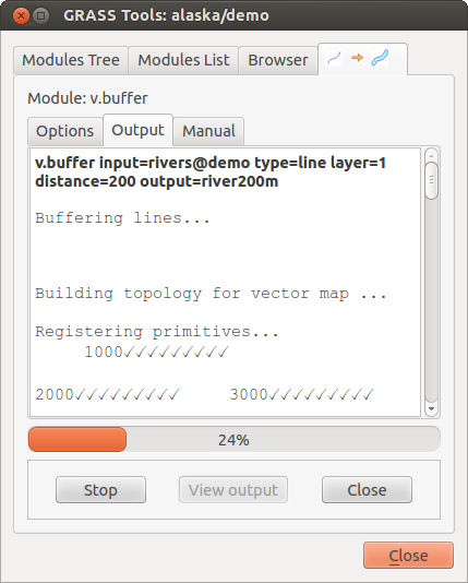
GRASS ツールボックス出力

The Output tab provides information about the output status of the module. When you click the [Run] button, the module switches to the Output tab and you see information about the analysis process. If all works well, you will finally see a Successfully finished message.

マニュアル

Figure GRASS module 3:

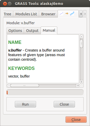
GRASSツールボックスモジュールマニュアル

The Manual tab shows the HTML help page of the GRASS module. You can use it to check further module parameters and flags or to get a deeper knowledge about the purpose of the module. At the end of each module manual page, you see further links to the Main Help index, the Thematic index and the Full index. These links provide the same information as the module g.manual.

ちなみに

結果をすぐ表示

もし計算結果をすぐにマップキャンバスに表示したい場合モジュールタブの一番下にある ‘View Output’ ボタンを利用できます.

GRASSモジュールの例¶

以下の例はいくつかの GRASS モジュールの力をデモンストレートします.

等高線の作成¶

The first example creates a vector contour map from an elevation raster (DEM). Here, it is assumed that you have the Alaska LOCATION set up as explained in section GRASS LOCATIONへデータをインポート.

• First, open the location by clicking the ^{Open mapset} button and choosing the Alaska location.

• ここで ^{Add GRASS raster layer} をクリックして gtopo30 標高ラスタをロードします,そして gtopo30 をdemoロケーションから選択します.

• Now open the Toolbox with the ^{Open GRASS tools} button.
• In the list of tool categories, double-click Raster ‣ Surface Management ‣ Generate vector contour lines.
• Now a single click on the tool r.contour will open the tool dialog as explained above (see GRASSモジュールを使用します). The gtopo30 raster should appear as the Name of input raster.
• Type into the Increment between Contour levels the value 100. (This will create contour lines at intervals of 100 meters.)
• Type into the Name for output vector map the name ctour_100.
• Click [Run] to start the process. Wait for several moments until the message Successfully finished appears in the output window. Then click [View Output] and [Close].

Since this is a large region, it will take a while to display. After it finishes rendering, you can open the layer properties window to change the line color so that the contours appear clearly over the elevation raster, as in ベクタプロパティダイアログ.

Next, zoom in to a small, mountainous area in the center of Alaska. Zooming in close, you will notice that the contours have sharp corners. GRASS offers the v.generalize tool to slightly alter vector maps while keeping their overall shape. The tool uses several different algorithms with different purposes. Some of the algorithms (i.e., Douglas Peuker and Vertex Reduction) simplify the line by removing some of the vertices. The resulting vector will load faster. This process is useful when you have a highly detailed vector, but you are creating a very small-scale map, so the detail is unnecessary.

ちなみに

シンプル化ツール

Note that the QGIS fTools plugin has a Simplify geometries ‣ tool that works just like the GRASS v.generalize Douglas-Peuker algorithm.

However, the purpose of this example is different. The contour lines created by r.contour have sharp angles that should be smoothed. Among the v.generalize algorithms, there is Chaiken’s, which does just that (also Hermite splines). Be aware that these algorithms can add additional vertices to the vector, causing it to load even more slowly.

• Open the GRASS Toolbox and double-click the categories Vector ‣ Develop map ‣ Generalization, then click on the v.generalize module to open its options window.
• Check that the ‘ctour_100’ vector appears as the Name of input vector.
• From the list of algorithms, choose Chaiken’s. Leave all other options at their default, and scroll down to the last row to enter in the field Name for output vector map ‘ctour_100_smooth’, and click [Run].
• The process takes several moments. Once Successfully finished appears in the output windows, click [View output] and then [Close].
• You may change the color of the vector to display it clearly on the raster background and to contrast with the original contour lines. You will notice that the new contour lines have smoother corners than the original while staying faithful to the original overall shape.

Figure GRASS module 4:

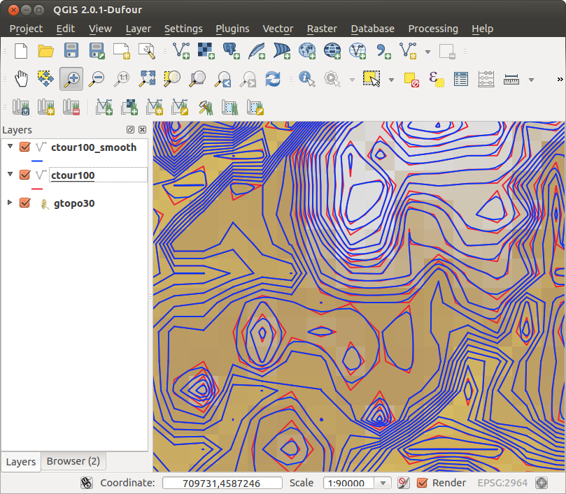
GRASS module v.generalize to smooth a vector map

ちなみに

その他にr.contourも使えます

The procedure described above can be used in other equivalent situations. If you have a raster map of precipitation data, for example, then the same method will be used to create a vector map of isohyetal (constant rainfall) lines.

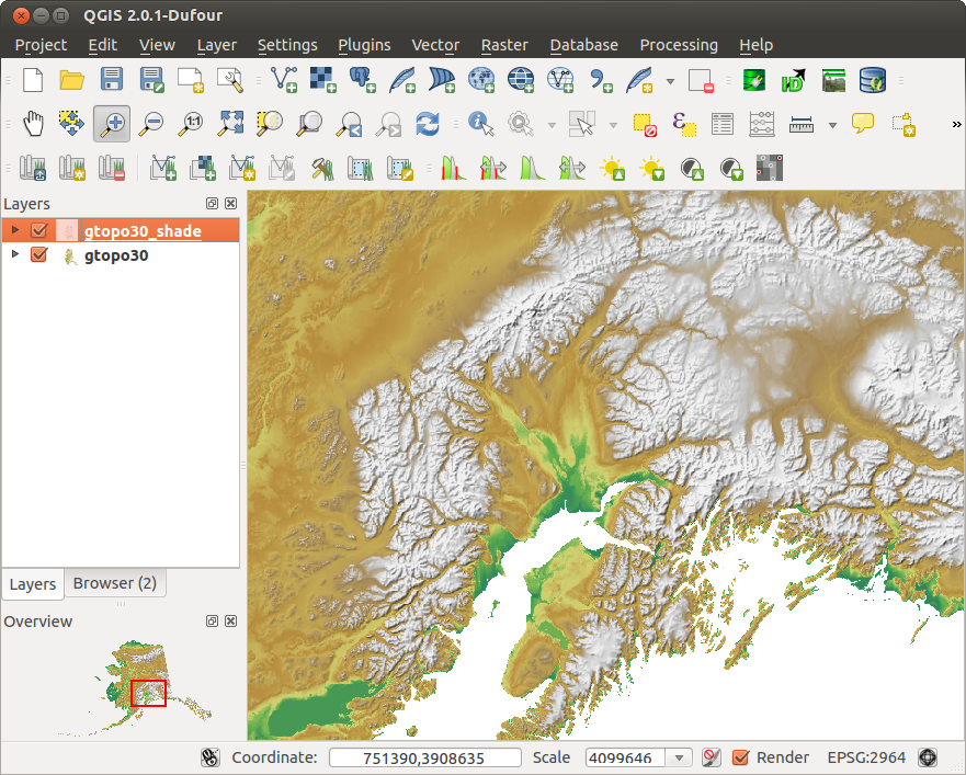
陰影3D効果の作成¶

Several methods are used to display elevation layers and give a 3-D effect to maps. The use of contour lines, as shown above, is one popular method often chosen to produce topographic maps. Another way to display a 3-D effect is by hillshading. The hillshade effect is created from a DEM (elevation) raster by first calculating the slope and aspect of each cell, then simulating the sun’s position in the sky and giving a reflectance value to each cell. Thus, you get sun-facing slopes lighted; the slopes facing away from the sun (in shadow) are darkened.

• Begin this example by loading the gtopo30 elevation raster. Start the GRASS Toolbox, and under the Raster category, double-click to open Spatial analysis ‣ Terrain analysis.

• それからモジュールをオープンするために r.shaded.relief をクリックして下さい.

• Change the azimuth angle 270 to 315.

• 新しいヒルシェードラスタとして gtopo30_shade と入力して [Run] をクリックして下さい.

• プロセスが完了するとヒルシェードラスタが地図に追加されます.これはグレイスケールで表示されます.

• To view both the hillshading and the colors of the gtopo30 together, move the hillshade map below the gtopo30 map in the table of contents, then open the Properties window of gtopo30, switch to the Transparency tab and set its transparency level to about 25%.

You should now have the gtopo30 elevation with its colormap and transparency setting displayed above the grayscale hillshade map. In order to see the visual effects of the hillshading, turn off the gtopo30_shade map, then turn it back on.

GRASS shellの使用

The GRASS plugin in QGIS is designed for users who are new to GRASS and not familiar with all the modules and options. As such, some modules in the Toolbox do not show all the options available, and some modules do not appear at all. The GRASS shell (or console) gives the user access to those additional GRASS modules that do not appear in the Toolbox tree, and also to some additional options to the modules that are in the Toolbox with the simplest default parameters. This example demonstrates the use of an additional option in the r.shaded.relief module that was shown above.

Figure GRASS module 5:

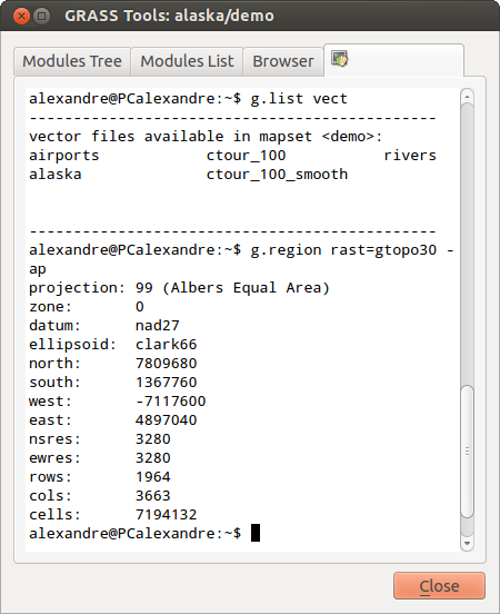
GRASSシェル, r.shaded.relief モジュール

The module r.shaded.relief can take a parameter zmult, which multiplies the elevation values relative to the X-Y coordinate units so that the hillshade effect is even more pronounced.

• Load the gtopo30 elevation raster as above, then start the GRASS Toolbox and click on the GRASS shell. In the shell window, type the command r.shaded.relief map=gtopo30 shade=gtopo30_shade2 azimuth=315 zmult=3 and press [Enter].
• After the process finishes, shift to the Browse tab and double-click on the new gtopo30_shade2 raster to display it in QGIS.
• As explained above, move the shaded relief raster below the gtopo30 raster in the table of contents, then check the transparency of the colored gtopo30 layer. You should see that the 3-D effect stands out more strongly compared with the first shaded relief map.

Figure GRASS module 6:

GRASSモジュール r.shaded.relief で作成した陰影図の表示

ベクターマップによるラスター統計¶

次の例はGRASS モジュールがラスタデータを集計してベクタマップのそれぞれのポリゴンのカラムに統計値を追加するものです.

• 再び Alaska データを使います, GRASS LOCATIONへデータをインポート を参照して shapefiles ディレクトリからshapefile treesをGRASSにインポートして下さい.

• Now an intermediate step is required: centroids must be added to the imported trees map to make it a complete GRASS area vector (including both boundaries and centroids).

• ツールボックスで Vector ‣ Manage features, を選択して v.centroids モジュールを開いて下さい.

• Enter as the output vector map ‘forest_areas’ and run the module.
• Now load the forest_areas vector and display the types of forests - deciduous, evergreen, mixed - in different colors: In the layer Properties window, Symbology tab, choose from Legend type ‘Unique value’ and set the Classification field to ‘VEGDESC’. (Refer to the explanation of the symbology tab in スタイルメニュー of the vector section.)

• 次に GRASS ツールボックスを再オープンして Vector ‣ Vector update を他の地図で開いて下さい.

• v.rast.stats モジュールをクリックして. gtopo30, と forest_areas と入力して下さい.

• Only one additional parameter is needed: Enter column prefix elev, and click [Run]. This is a computationally heavy operation, which will run for a long time (probably up to two hours).
• Finally, open the forest_areas attribute table, and verify that several new columns have been added, including elev_min, elev_max, elev_mean, etc., for each forest polygon.

GRASS LOCATION ブラウザの作業¶

Another useful feature inside the GRASS Toolbox is the GRASS LOCATION browser. In figure_grass_module_7, you can see the current working LOCATION with its MAPSETs.

In the left browser windows, you can browse through all MAPSETs inside the current LOCATION. The right browser window shows some meta-information for selected raster or vector layers (e.g., resolution, bounding box, data source, connected attribute table for vector data, and a command history).

Figure GRASS module 7:

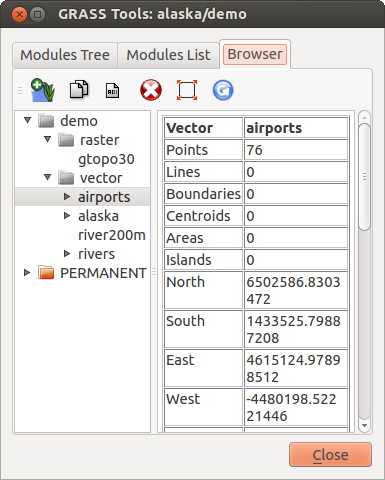
GRASS LOCATION ブラウザ

The toolbar inside the Browser tab offers the following tools to manage the selected LOCATION:

• 選択した地図をキャンバスへ追加

• 選択した地図をコピー

• 選択した地図の名前変更

• 選択した地図を削除

• 領域設定を選択した地図に合わせる

• ブラウザウィンドウの表示更新

The Rename selected map and Delete selected map only work with maps inside your currently selected MAPSET. All other tools also work with raster and vector layers in another MAPSET.

<?xml version="1.0" encoding="UTF-8"?>
<!DOCTYPE qgisgrassmodule SYSTEM "http://mrcc.com/qgisgrassmodule.dtd">

<qgisgrassmodule label="Vector buffer" module="v.buffer">
        <option key="input" typeoption="type" layeroption="layer" />
        <option key="buffer"/>
        <option key="output" />
</qgisgrassmodule>