ベクタプロパティダイアログ¶

スタイルメニュー¶

スタイルメニューではベクタデータをレンダリングとシンボライジングを行うための包括的ツールを提供します. レイヤレンダリング ‣ ツールはすべてのベクタデータに対して共通で利用でき異なる種類のベクタデータ向けの特別シンボライズツールもあります.

レンダラー¶

The renderer is responsible for drawing a feature together with the correct symbol. There are four types of renderers: single symbol, categorized, graduated and rule-based. There is no continuous color renderer, because it is in fact only a special case of the graduated renderer. The categorized and graduated renderers can be created by specifying a symbol and a color ramp - they will set the colors for symbols appropriately. For point layers, there is a point displacement renderer available. For each data type (points, lines and polygons), vector symbol layer types are available. Depending on the chosen renderer, the Style menu provides different additional sections. On the bottom right of the symbology dialog, there is a [Symbol] button, which gives access to the Style Manager (see Presentation). The Style Manager allows you to edit and remove existing symbols and add new ones.

After having made any needed changes, the symbol can be added to the list of current style symbols (using [Symbol] Save in symbol library), and then it can easily be used in the future. Furthermore, you can use the [Save Style] button to save the symbol as a QGIS layer style file (.qml) or SLD file (.sld). SLDs can be exported from any type of renderer – single symbol, categorized, graduated or rule-based – but when importing an SLD, either a single symbol or rule-based renderer is created. That means that categorized or graduated styles are converted to rule-based. If you want to preserve those renderers, you have to stick to the QML format. On the other hand, it can be very handy sometimes to have this easy way of converting styles to rule-based.

If you change the renderer type when setting the style of a vector layer the settings you made for the symbol will be maintained. Be aware that this procedure only works for one change. If you repeat changing the renderer type the settings for the symbol will get lost.

If the datasource of the layer is a database (PostGIS or Spatialite for example), you can save your layer style inside a table of the database. Just clic on :guilabel:` Save Style` comboxbox and choose Save in database item then fill in the dialog to define a style name, add a description, an ui file and if the style is a default style. When loading a layer from the database, if a style already exists for this layer, QGIS will load the layer and its style. You can add several style in the database. Only one will be the default style anyway.

Figure Vector Properties 2:

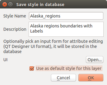
Save Style in database Dialog

ちなみに

複数シンボルを選択して変更する

シンボロジでは複数のシンボルを選択して右クリックでそれらの色,透過度,サイズや太さを変更できます.

単一シンボルレンダラ

シングルシンボルレンダラはあるレイヤの全ての地物を単一のユーザ定義シンボルで描画するために利用されます. スタイル メニューでプロパティの調節ができます, それらの内容は部分的にはレイヤタイプに依存しますが,すべてのタイプで以下のダイアログのような構造を共有しています. メニューの上部左側の部分には設定されているシンボルのプレビューが描画されます. メニューの右側には現在のスタイルですでに定義されているシンボルリストが表示され,それらを選択して利用することができます. 右側にあるメニューを使ってカレントシンボルを編集することができます.

If you click on the first level in the Symbol layers dialog on the left side, it’s possible to define basic parameters like Size, Transparency, color and Rotation. Here, the layers are joined together.

Figure Symbology 1:

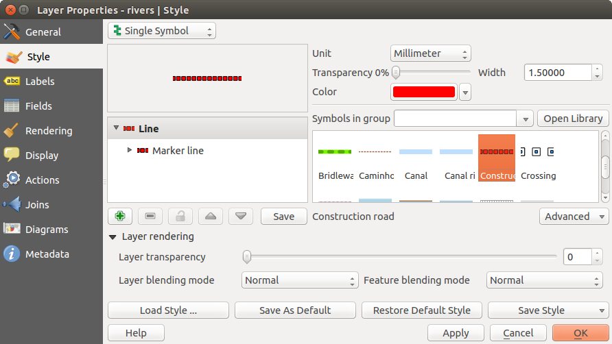
単一シンボルラインプロパティ

カテゴライズドレンダラ

カテゴライズドレンダラはレイヤのすべての地物を単一のユーザ指定シンボルを使って選択地物の属性の値によって決められる色で描画します. スタイル メニューで選択できます:

• The attribute (using the Column listbox or the Set column expression function, see Expressions)

• シンボル(シンボルダイアログを利用)

• The colors (using the color Ramp listbox)

Then click on Classify button to create classes from the distinct value of the attribute column. Each classes can be disabled unchecking the checkbox at the left of the class name.

You can change symbol, value and/or label of the clic, just double clicking on the item you want to change.

Right-clic shows a contextual menu to Copy/Paste, Change color, Change transparency, Change output unit, Change symbol width.

ダイアログの右下にある [Advanced] ボタンを使うとフィールドに回転角とサイズ,スケールの情報を格納できます. メニューの中央のリストにはシンボルレンダリングのために選択されている属性値がリストされます.

figure_symbology_2 では QGIS サンプルデータセットの riversレイヤを使ったカテゴリレンダリングダイアログの例が表示されています.

Figure Symbology 2:

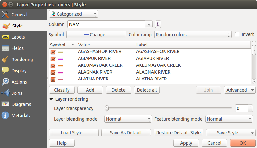
カテゴライズドシンボライジングオプション

グラヂュエイデッドレンダラ

The Graduated Renderer is used to render all the features from a layer, using a single user-defined symbol whose color reflects the assignment of a selected feature’s attribute to a class.

Figure Symbology 4:

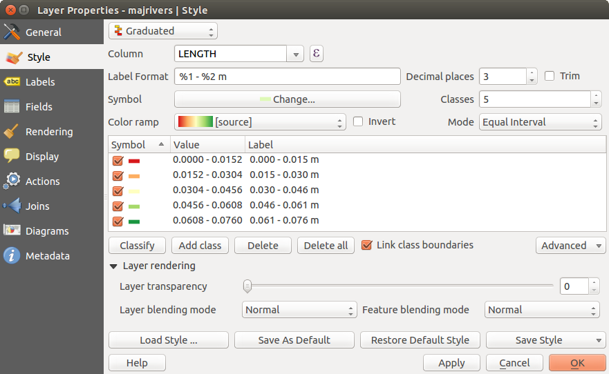
グラヂュエイデッドシンボルオプション

カテゴライズレンダラと同じように一般レンダラでは回転とサイズスケールの値を特定のカラムに定義できます.

また、カテゴライズドレンダラと同じように スタイル タブで選択できます:

• The attribute (using the Column listbox or the Set column expression function, see Expressions chapter)

• シンボル(シンボルプロパティボタンを利用)

• The colors (using the color Ramp list)

さらにクラスの数とクラス内で地物をどのように分類するか(モードメニューを使用)指定できます.利用できるモードは次のとおりです:

• Equal Interval: each class has the same size (e.g. values from 0 to 16 and 4 classes, each class has a size of 4);
• Quantile: each class will have the same number of element inside (the idea of a boxplot);
• Natural Breaks (Jenks): the variance within each class is minimal while the variance between classes is maximal;
• Standard Deviation: classes are built depending on the standard deviation of the values;
• Pretty Breaks: the same of natural breaks but the extremes number of each class are integers.

The listbox in the center part of the Style menu lists the classes together with their ranges, labels and symbols that will be rendered.

Click on Classify button to create classes using the choosen mode. Each classes can be disabled unchecking the checkbox at the left of the class name.

You can change symbol, value and/or label of the clic, just double clicking on the item you want to change.

Right-clic shows a contextual menu to Copy/Paste, Change color, Change transparency, Change output unit, Change symbol width.

figure_symbology_4 の例は QGIS サンプルデータセットのリバーレイヤを利用した段彩レンダリングダイアログです.

ちなみに

式を利用した主題図

Categorized and graduated thematic maps can now be created using the result of an expression. In the properties dialog for vector layers, the attribute chooser has been augmented with a Set column expression function. So now you no longer need to write the classification attribute to a new column in your attribute table if you want the classification attribute to be a composite of multiple fields, or a formula of some sort.

ルールベースレンダリング

ルールベースレンダラは選択された地物の属性をクラス分けする規則に基づいた描画方法でレイヤのすべての地物を描画するために利用されています. 規則は SQL 構文に基づきます. ダイアログではフィルターやスケールでルールをグループ化できます,そして必要ならばシンボルレベルを有効にしたり最初にマッチしたルールのみ利用することもできます.

figure_symbology_5 の例は QGIS サンプルデータセットのリバーレイヤを利用したルールベースドレンダリングダイアログです.

To create a rule, activate an existing row by double-clicking on it, or click on ‘+’ and click on the new rule. In the Rule properties dialog, you can define a label for the rule. Press the button to open the expression string builder. In the Function List, click on Fields and Values to view all attributes of the attribute table to be searched. To add an attribute to the field calculator Expression field, double click its name in the Fields and Values list. Generally, you can use the various fields, values and functions to construct the calculation expression, or you can just type it into the box (see Expressions). You can create a new rule by copying and pasting an existing rule with the right mouse button. You can also use the ‘ELSE’ rule that will be run if none of the other rules on that level match. Since QGIS 2.6 the label for the rules appears in a pseudotree in the map legend. Just double-klick the rules in the map legend and the Style menu of the layer properties appears showing the rule that is the background for the symbol in the pseudotree.

Figure Symbology 5:

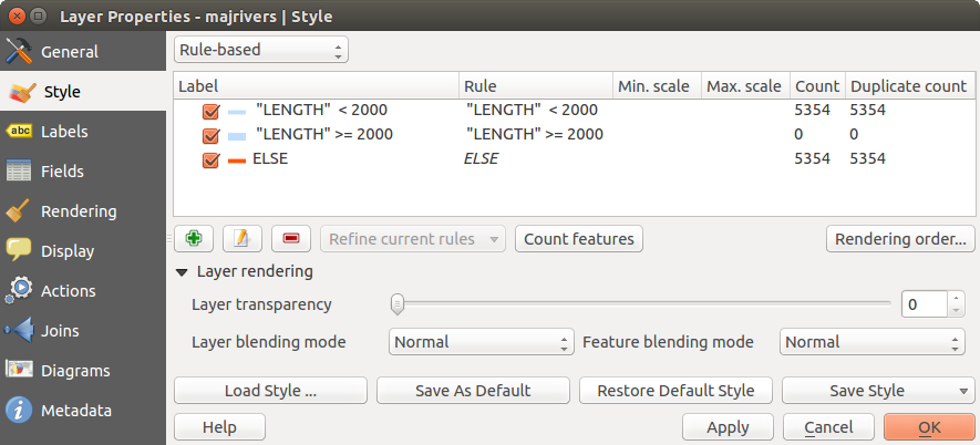
ルールベースドシンボライズドオプション

ポイント移動

ポイント移動レンダラはもしそれらがすべて同じ位置にあったとしてもポイントレイヤの地物を描画するのに利用されます. 同じ位置のポイントを描画する場合は中心のシンボルのまわりに円形に移動して描画されます.

Figure Symbology 6:

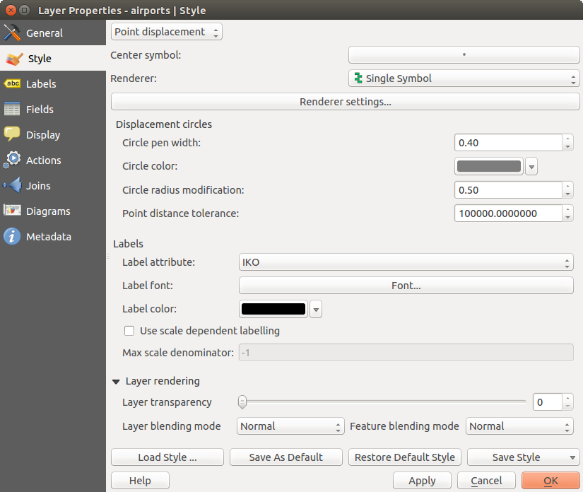
ポイント移動ダイアログ

ちなみに

ベクタシンボロジーのエキスポート

You have the option to export vector symbology from QGIS into Google *.kml, *.dxf and MapInfo *.tab files. Just open the right mouse menu of the layer and click on Save selection as ‣ to specify the name of the output file and its format. In the dialog, use the Symbology export menu to save the symbology either as Feature symbology ‣ or as Symbol layer symbology ‣. If you have used symbol layers, it is recommended to use the second setting.

Inverted Polygon

Inverted polygon renderer allows user to define a symbol to fill in outside of the layer’s polygons. As before you can select a subrenderers. These subrenderers are the same as for the main renderers.

Figure Symbology 7:

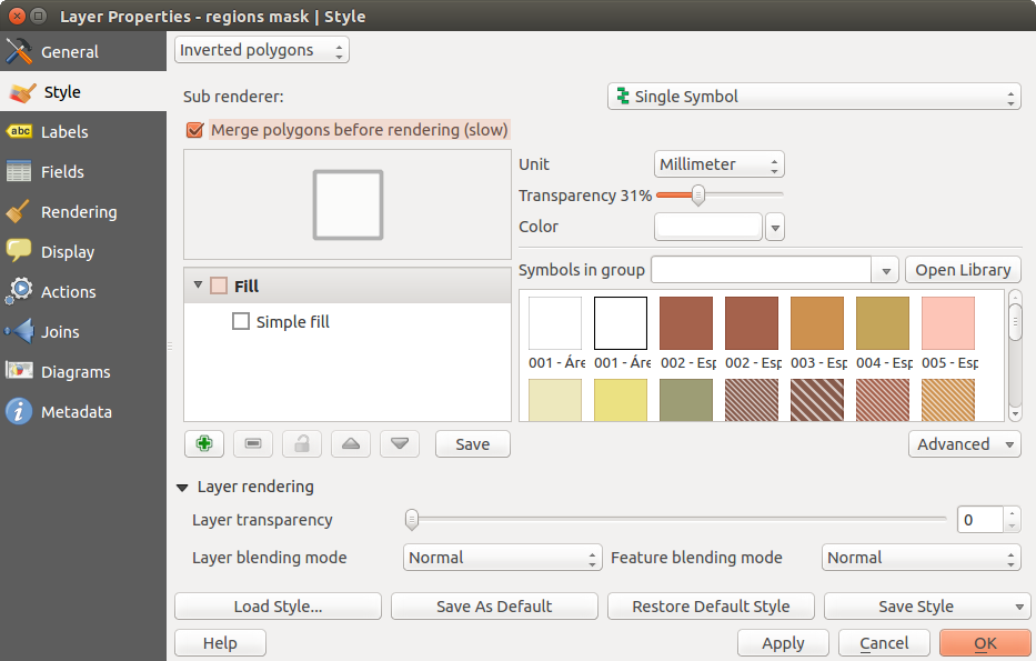
Inverted Polygon dialog

Color Picker¶

Regardless the type of style to be used, the select color dialog will show when you click to choose a color - either border or fill color. This dialog has four different tabs which allow you to select colors by ^{color ramp}, ^{color wheel}, ^{color swatches} or ^{color picker}.

Whatever method you use, the selected color is always described through color sliders for HSV (Hue, Saturation, Value) and RGB (Red, Green, Blue) values. There is also an opacity slider to set transparency level. On the lower left part of the dialog you can see a comparison between the current and the new color you are presently selecting and on the lower right part you have the option to add the color you just tweaked into a color slot button.

Figure color picker 1:

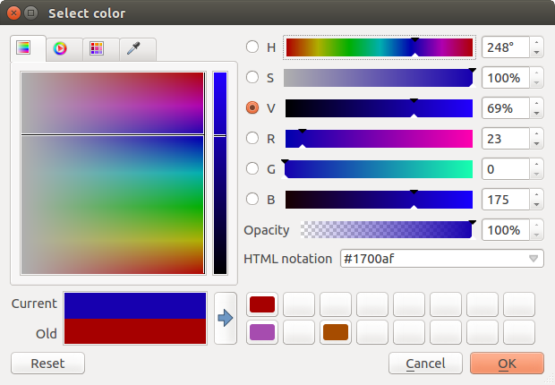
Color picker ramp tab

With ^{color ramp} or with ^{color wheel}, you can browse to all possible color combinations. There are other possibilities though. By using color swatches you can choose from a preselected list. This selected list is populated with one of three methods: Recent colors, Standard colors or Project colors

Figure color picker 2:

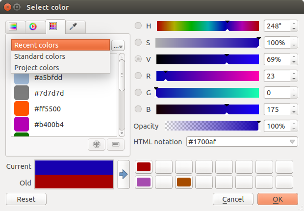
Color picker swatcher tab

Another option is to use the ^{color picker} which allows you to sample a color from under your mouse pointer at any part of QGIS or even from another application by pressing the space bar. Please note that the color picker is OS dependent and is currently not supported by OSX.

ちなみに

quick color picker + copy/paste colors

You can quickly choose from Recent colors, from Standard colors or simply copy or paste a color by clicking the drop-down arrow that follows a current color box.

Figure color picker 3:

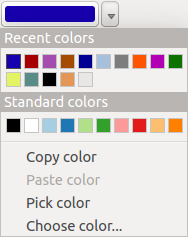
Quick color picker menu

ラベルメニュー¶

The ^Labels core application provides smart labeling for vector point, line and polygon layers, and it only requires a few parameters. This new application also supports on-the-fly transformed layers. The core functions of the application have been redesigned. In QGIS, there are a number of other features that improve the labeling. The following menus have been created for labeling the vector layers:

• テキスト

• 整形

• バッファ

• 背景

• 影

• 配置

• 描画

新しいメニューが多彩なベクタレイヤでどのように利用されるか見てみましょう.

ポイントレイヤのラベリング

Start QGIS and load a vector point layer. Activate the layer in the legend and click on the ^{Layer Labeling Options} icon in the QGIS toolbar menu.

The first step is to activate the Label this layer with checkbox and select an attribute column to use for labeling. Click if you want to define labels based on expressions - See labeling_with_expressions.

以下のステップはドロップダウンメニューの隣にある Data defined override 機能を使わない単純なラベル機能の説明です.

You can define the text style in the Text menu (see Figure_labels_1 ). Use the Type case option to influence the text rendering. You have the possibility to render the text ‘All uppercase’, ‘All lowercase’ or ‘Capitalize first letter’. Use the blend modes to create effects known from graphics programs (see blend_modes).

In the Formatting menu, you can define a character for a line break in the labels with the ‘Wrap on character’ function. Use the Formatted numbers option to format the numbers in an attribute table. Here, decimal places may be inserted. If you enable this option, three decimal places are initially set by default.

To create a buffer, just activate the Draw text buffer checkbox in the Buffer menu. The buffer color is variable. Here, you can also use blend modes (see blend_modes).

If the color buffer’s fill checkbox is activated, it will interact with partially transparent text and give mixed color transparency results. Turning off the buffer fill fixes that issue (except where the interior aspect of the buffer’s stroke intersects with the text’s fill) and also allows you to make outlined text.

In the Background menu, you can define with Size X and Size Y the shape of your background. Use Size type to insert an additional ‘Buffer’ into your background. The buffer size is set by default here. The background then consists of the buffer plus the background in Size X and Size Y. You can set a Rotation where you can choose between ‘Sync with label’, ‘Offset of label’ and ‘Fixed’. Using ‘Offset of label’ and ‘Fixed’, you can rotate the background. Define an Offset X,Y with X and Y values, and the background will be shifted. When applying Radius X,Y, the background gets rounded corners. Again, it is possible to mix the background with the underlying layers in the map canvas using the Blend mode (see blend_modes).

Use the Shadow menu for a user-defined Drop shadow. The drawing of the background is very variable. Choose between ‘Lowest label component’, ‘Text’, ‘Buffer’ and ‘Background’. The Offset angle depends on the orientation of the label. If you choose the Use global shadow checkbox, then the zero point of the angle is always oriented to the north and doesn’t depend on the orientation of the label. You can influence the appearance of the shadow with the Blur radius. The higher the number, the softer the shadows. The appearance of the drop shadow can also be altered by choosing a blend mode (see blend_modes).

Choose the Placement menu for the label placement and the labeling priority. Using the Offset from point setting, you now have the option to use Quadrants to place your label. Additionally, you can alter the angle of the label placement with the Rotation setting. Thus, a placement in a certain quadrant with a certain rotation is possible.

In the Rendering menu, you can define label and feature options. Under Label options, you find the scale-based visibility setting now. You can prevent QGIS from rendering only selected labels with the Show all labels for this layer (including colliding labels) checkbox. Under Feature options, you can define whether every part of a multipart feature is to be labeled. It’s possible to define whether the number of features to be labeled is limited and to Discourage labels from covering features.

Figure Labels 1:

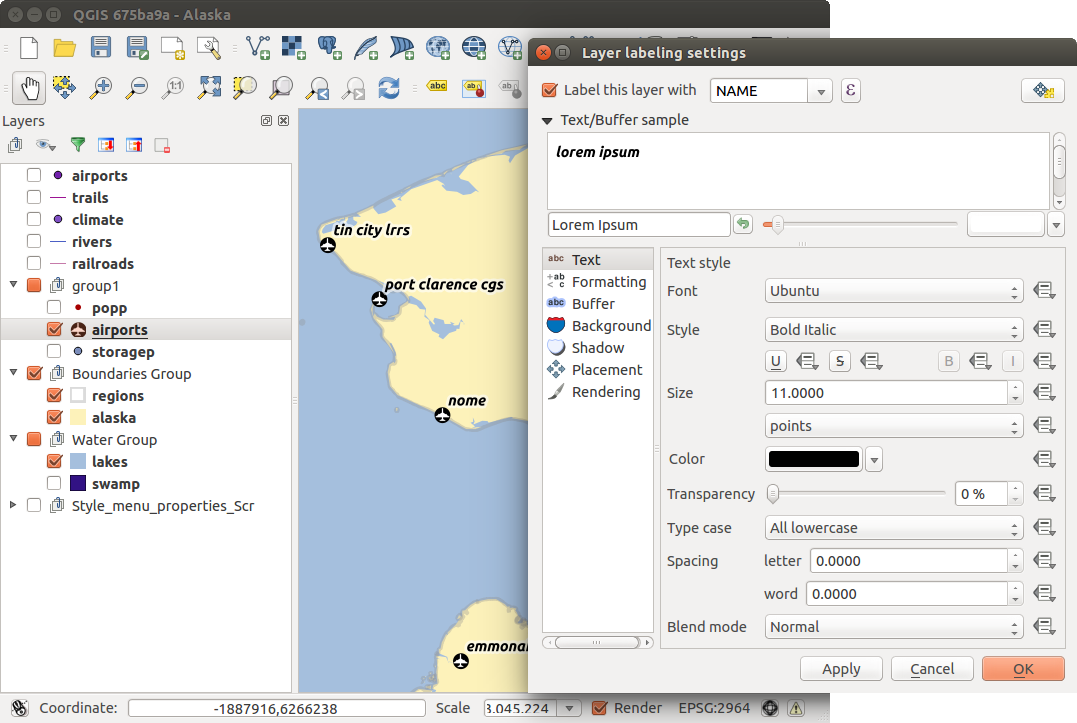
ベクタポイントレイヤのスマートラベリング

ラインレイヤのラベリング

The first step is to activate the Label this layer checkbox in the Label settings tab and select an attribute column to use for labeling. Click if you want to define labels based on expressions - See labeling_with_expressions.

After that, you can define the text style in the Text menu. Here, you can use the same settings as for point layers.

Also, in the Formatting menu, the same settings as for point layers are possible.

The Buffer menu has the same functions as described in section labeling_point_layers.

The Background menu has the same entries as described in section labeling_point_layers.

さらに Shadow メニューにはセクション labeling_point_layers で記述されているのと同じエントリがあります.

In the Placement menu, you find special settings for line layers. The label can be placed Parallel, Curved or Horizontal. With the Parallel and Curved option, you can define the position Above line, On line and Below line. It’s possible to select several options at once. In that case, QGIS will look for the optimal position of the label. Remember that here you can also use the line orientation for the position of the label. Additionally, you can define a Maximum angle between curved characters when selecting the Curved option (see Figure_labels_2 ).

You can set up a minimum distance for repeating labels. Distance can be in mm or in map units.

Some Placement setup will display more options, for example, Curved and Parallel Placements will allow the user to set up the position of the label (above, belw or on the line), distance from the line and for Curved, the user can also setup inside/outside max angle between curved label.

The Rendering menu has nearly the same entries as for point layers. In the Feature options, you can now Suppress labeling of features smaller than.

Figure Labels 2:

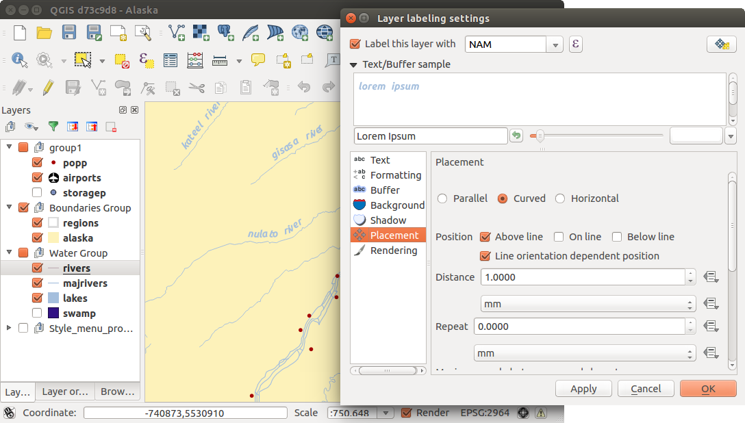
ベクタラインレイヤのスマートラベリング

ポリゴンレイヤのラベリング

The first step is to activate the Label this layer checkbox and select an attribute column to use for labeling. Click if you want to define labels based on expressions - See labeling_with_expressions.

In the Text menu, define the text style. The entries are the same as for point and line layers.

The Formatting menu allows you to format multiple lines, also similar to the cases of point and line layers.

ポイントおよびラインレイヤで、 バッファ メニューでテキストバッファを作成できます。

Use the Background menu to create a complex user-defined background for the polygon layer. You can use the menu also as with the point and line layers.

The entries in the Shadow menu are the same as for point and line layers.

In the Placement menu, you find special settings for polygon layers (see Figure_labels_3). Offset from centroid, Horizontal (slow), Around centroid, Free and Using perimeter are possible.

In the Offset from centroid settings, you can specify if the centroid is of the visible polygon or whole polygon. That means that either the centroid is used for the polygon you can see on the map or the centroid is determined for the whole polygon, no matter if you can see the whole feature on the map. You can place your label with the quadrants here, and define offset and rotation. The Around centroid setting makes it possible to place the label around the centroid with a certain distance. Again, you can define visible polygon or whole polygon for the centroid. With the Using perimeter settings, you can define a position and a distance for the label. For the position, Above line, On line, Below line and Line orientation dependent position are possible.

Related to the choose of Label Placement, several options will appear. As for Point Placement you can choose the distance for the polygon outline, repeat the label around the polygon perimeter.

レンダリング メニューでの入力はラインレイヤと同じです。 地物オプション で これより小さいラベリングを行わない を使用できます。

Figure Labels 3:

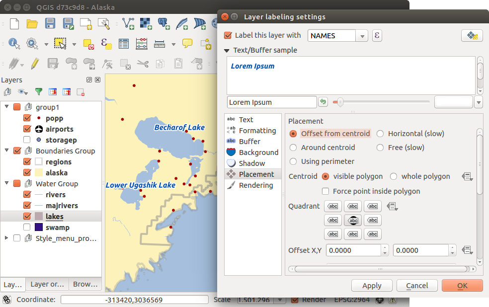
ベクタポイントレイヤのスマートラベリング

式に基づいたラベルの定義

QGIS allows to use expressions to label features. Just click the icon in the ^Labels menu of the properties dialog. In figure_labels_4 you see a sample expression to label the alaska regions with name and area size, based on the field ‘NAME_2’, some descriptive text and the function ‘$area()’ in combination with ‘format_number()’ to make it look nicer.

Figure Labels 4:

ラベリング用の式利用

Expression based labeling is easy to work with. All you have to take care of is, that you need to combine all elements (strings, fields and functions) with a string concatenation sign ‘||’ and that fields a written in “double quotes” and strings in ‘single quotes’. Let’s have a look at some examples:

 # label based on two fields 'name' and 'place' with a comma as separater
 "name" || ', ' || "place"

 -> John Smith, Paris

 # label based on two fields 'name' and 'place' separated by comma
 'My name is ' || "name" || 'and I live in ' || "place"

 -> My name is John Smith and I live in Paris

 # label based on two fields 'name' and 'place' with a descriptive text
 # and a line break (\n)
 'My name is ' || "name" || '\nI live in ' || "place"

 -> My name is John Smith
    I live in Paris

 # create a multi-line label based on a field and the $area function
 # to show the place name and its area size based on unit meter.
 'The area of ' || "place" || 'has a size of ' || $area || 'm²'

 -> The area of Paris has a size of 105000000 m²

 # create a CASE ELSE condition. If the population value in field
 # population is <= 50000 it is a town, otherwise a city.
 'This place is a ' || CASE WHEN "population <= 50000" THEN 'town' ELSE 'city' END

-> This place is a town

As you can see in the expression builder, you have hundreds if functions available to create simple and very complex expressions to label your data in QGIS. See Expressions chapter for more information and example on expressions.

ラベルのデータ定義オーバーライドの利用

With the data-defined override functions, the settings for the labeling are overridden by entries in the attribute table. You can activate and deactivate the function with the right-mouse button. Hover over the symbol and you see the information about the data-defined override, including the current definition field. We now describe an example using the data-defined override function for the ^{Move label} function (see figure_labels_5 ).

1. Import lakes.shp from the QGIS sample dataset.

2. レイヤをダブルクリックしてレイヤプロパティを開いて下さい. Labels と Placement をクリックして下さい. Offset from centroid を選択して下さい.

3. Look for the Data defined entries. Click the icon to define the field type for the Coordinate. Choose ‘xlabel’ for X and ‘ylabel’ for Y. The icons are now highlighted in yellow.

4. 湖へズーム

5. Go to the Label toolbar and click the icon. Now you can shift the label manually to another position (see figure_labels_6 ). The new position of the label is saved in the ‘xlabel’ and ‘ylabel’ columns of the attribute table.

Figure Labels 5:

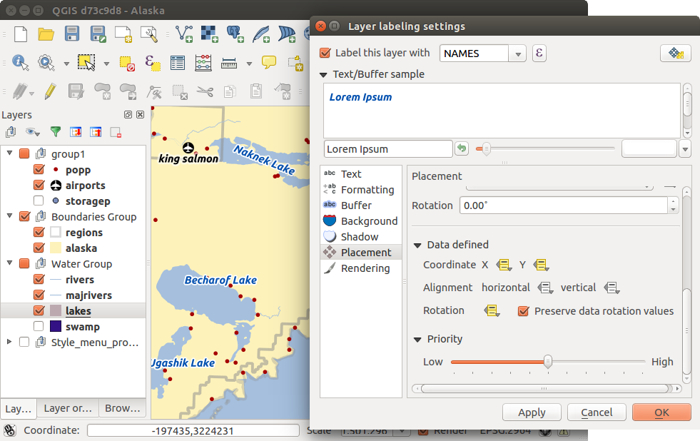
データ定義でオーバーライドされたベクタポリゴンレイヤのラベリング

Figure Labels 6:

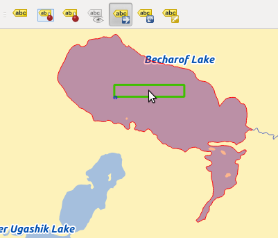
ラベルの移動

フィールドメニュー¶

Within the Fields menu, the field attributes of the selected dataset can be manipulated. The buttons ^{New Column} and ^{Delete Column} can be used when the dataset is in ^{Editing mode}.

編集ウィジェット

Figure Fields 1:

属性カラムのための編集ウィジェット選択ダイアログ

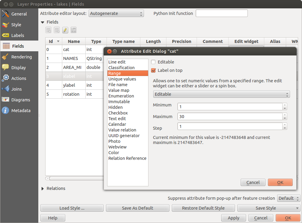
Within the Fields menu, you also find an edit widget column. This column can be used to define values or a range of values that are allowed to be added to the specific attribute table column. If you click on the [edit widget] button, a dialog opens, where you can define different widgets. These widgets are:

• Checkbox: Displays a checkbox, and you can define what attribute is added to the column when the checkbox is activated or not.

• 分類: , プロパティの スタイル メニューで ‘固有値’ を凡例タイプとして選択している場合コンボボックスで分類を行う値を選択してください.

• Color: Displays a color button allowing user to choose a color from the color dialog window.
• Date/Time: Displays a line fields which can opens a calendar widget to enter a date, a time or both. Column type must be text. You can select a custom format, pop-up a calendar, etc.
• Enumeration: Opens a combo box with values that can be used within the columns type. This is currently only supported by the PostgreSQL provider.

• ファイル名: ダイアログにファイル選択を追加した簡素なファイル選択.

• Hidden: 隠れた属性カラムは見ることができません. ユーザーはそのコンテンツをみることができません.

• 写真: ピクチャのファイル名を含むフィールドです。フィールドの幅と高さが定義されます。

• Range: Allows you to set numeric values from a specific range. The edit widget can be either a slider or a spin box.
• Relation Reference: This widged lets you embed the feature form of the referenced layer on the feature form of the actual layer. See １対多リレーションの作成.
• Text edit (default): This opens a text edit field that allows simple text or multiple lines to be used. If you choose multiple lines you can also choose html content.
• Unique values: You can select one of the values already used in the attribute table. If ‘Editable’ is activated, a line edit is shown with autocompletion support, otherwise a combo box is used.

• UUID ジェネレータ:空の場合、読み取り専用のUUID (Universally Unique Identifiers) フィールドを生成します。

• Value map: A combo box with predefined items. The value is stored in the attribute, the description is shown in the combo box. You can define values manually or load them from a layer or a CSV file.

• 値のリレーション:コンボボックスでリレーションテーブルから値を提供します。レイヤ、キーカラム、値カラムで選択出来ます。

• Webview: Field contains a URL. The width and height of the field is variable.

With the Attribute editor layout, you can now define built-in forms for data entry jobs (see figure_fields_2). Choose ‘Drag and drop designer’ and an attribute column. Use the icon to create a category that will then be shown during the digitizing session (see figure_fields_3). The next step will be to assign the relevant fields to the category with the icon. You can create more categories and use the same fields again. When creating a new category, QGIS will insert a new tab for the category in the built-in form.

Other options in the dialog are ‘Autogenerate’ and ‘Provide ui-file’. ‘Autogenerate’ just creates editors for all fields and tabulates them. The ‘Provide ui-file’ option allows you to use complex dialogs made with the Qt-Designer. Using a UI-file allows a great deal of freedom in creating a dialog. For detailed information, see http://nathanw.net/2011/09/05/qgis-tips-custom-feature-forms-with-python-logic/.

QGIS dialogs can have a Python function that is called when the dialog is opened. Use this function to add extra logic to your dialogs. An example is (in module MyForms.py):

def open(dialog,layer,feature):
geom = feature.geometry()
control = dialog.findChild(QWidged,"My line edit")

: MyForms.open のような Python Init 関数を参照しましょう。

MyForms.py must live on PYTHONPATH, in .qgis2/python, or inside the project folder.

Figure Fields 2:

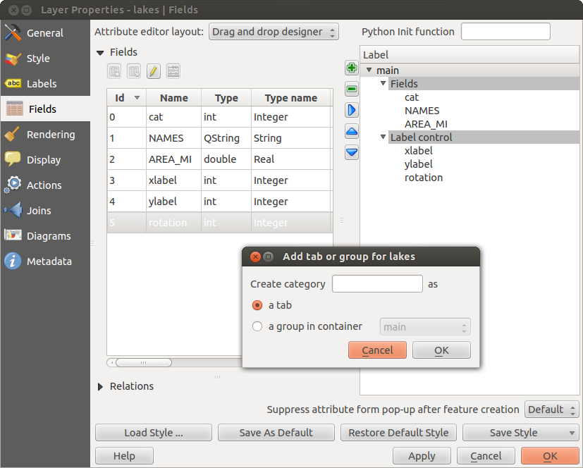
**属性編集レイアウト**でカテゴリを生成するダイアログ

Figure Fields 3:

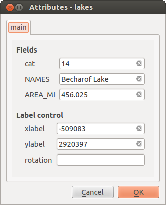
データ入力セッションでのビルトインフォームの結果

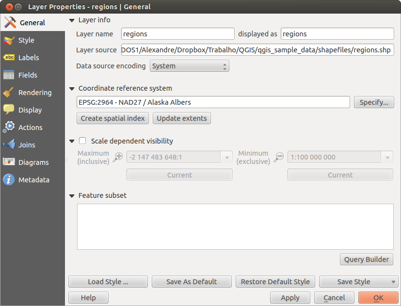
一般メニュー¶

このメニューはベクタレイヤの一般的な設定で利用します. ここには多くのオプションが利用できます:

レイヤ情報

• displayed as を使うとレイヤの表示名称を変更できます

• ベクタレイヤの Layer source を指定します

• Define the Data source encoding to define provider-specific options and to be able to read the file

空間参照システム

• Specify the coordinate reference system. Here, you can view or change the projection of the specific vector layer.
• Create a Spatial Index (only for OGR-supported formats)

• 領域の更新 レイヤの情報

• ベクタレイヤに指定されている投影方法を閲覧や変更したい場合は 指定 ... をクリックして下さい

縮尺に応じた表示設定

• You can set the Maximum (inclusive) and Minimum (exclusive) scale. The scale can also be set by the [Current] buttons.

地物サブセット

• With the [Query Builder] button, you can create a subset of the features in the layer that will be visualized (also refer to section クエリビルダー).

Figure General 1:

ベクタレイヤプロパティダイアログの一般情報メニュー

レンダリングメニュー¶

QGIS 2.2 introduces support for on-the-fly feature generalisation. This can improve rendering times when drawing many complex features at small scales. This feature can be enabled or disabled in the layer settings using the Simplify geometry option. There is also a new global setting that enables generalisation by default for newly added layers (see section オプション). Note: Feature generalisation may introduce artefacts into your rendered output in some cases. These may include slivers between polygons and inaccurate rendering when using offset-based symbol layers.

メニュー表示¶

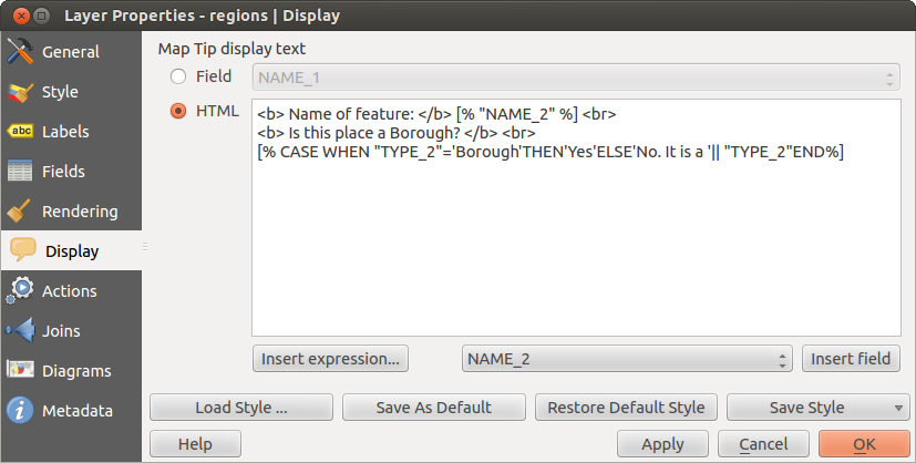
This menu is specifically created for Map Tips. It includes a new feature: Map Tip display text in HTML. While you can still choose a Field to be displayed when hovering over a feature on the map, it is now possible to insert HTML code that creates a complex display when hovering over a feature. To activate Map Tips, select the menu option View ‣ MapTips. Figure Display 1 shows an example of HTML code.

Figure Display 1:

マップチップのHTMLコード

Figure Display 2:

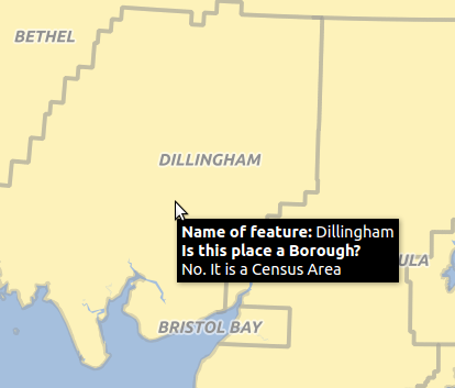
HTMLコードを使ったマップチップ

アクションメニュー¶

QGIS は、フィーチャの属性に基づいてアクションを実行する機能を提供します。これは、任意の数のアクションを実行するために使用することができ、例えば、地物の属性から引数を設定しプログラムを実行したり、Webレポーティングツールにパラメータを通します。

Figure Actions 1:

いくつかのサンプルアクションが表示されたアクションダイアログの概観

Actions are useful when you frequently want to run an external application or view a web page based on one or more values in your vector layer. They are divided into six types and can be used like this:

• Generic、Mac、WindowsとUnixのアクションが外部プロセスを開始します。

• Python アクションは Python 構文を実行します.

• GenericとPythonのアクションはどこでも見ることができます。

• Mac, Windows and Unix actions are visible only on the respective platform (i.e., you can define three ‘Edit’ actions to open an editor and the users can only see and execute the one ‘Edit’ action for their platform to run the editor).

There are several examples included in the dialog. You can load them by clicking on [Add default actions]. One example is performing a search based on an attribute value. This concept is used in the following discussion.

アクションの定義

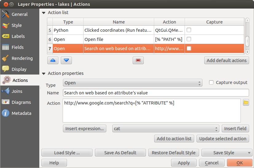
Attribute actions are defined from the vector Layer Properties dialog. To define an action, open the vector Layer Properties dialog and click on the Actions menu. Go to the Action properties. Select ‘Generic’ as type and provide a descriptive name for the action. The action itself must contain the name of the application that will be executed when the action is invoked. You can add one or more attribute field values as arguments to the application. When the action is invoked, any set of characters that start with a % followed by the name of a field will be replaced by the value of that field. The special characters %% will be replaced by the value of the field that was selected from the identify results or attribute table (see using_actions below). Double quote marks can be used to group text into a single argument to the program, script or command. Double quotes will be ignored if preceded by a backslash.

If you have field names that are substrings of other field names (e.g., col1 and col10), you should indicate that by surrounding the field name (and the % character) with square brackets (e.g., [%col10]). This will prevent the %col10 field name from being mistaken for the %col1 field name with a 0 on the end. The brackets will be removed by QGIS when it substitutes in the value of the field. If you want the substituted field to be surrounded by square brackets, use a second set like this: [[%col10]].

Using the Identify Features tool, you can open the Identify Results dialog. It includes a (Derived) item that contains information relevant to the layer type. The values in this item can be accessed in a similar way to the other fields by preceeding the derived field name with (Derived).. For example, a point layer has an X and Y field, and the values of these fields can be used in the action with %(Derived).X and %(Derived).Y. The derived attributes are only available from the Identify Results dialog box, not the Attribute Table dialog box.

2つの アクション例 が以下にあります:

• konqueror http://www.google.com/search?q=%nam
• konqueror http://www.google.com/search?q=%%

In the first example, the web browser konqueror is invoked and passed a URL to open. The URL performs a Google search on the value of the nam field from our vector layer. Note that the application or script called by the action must be in the path, or you must provide the full path. To be certain, we could rewrite the first example as: /opt/kde3/bin/konqueror http://www.google.com/search?q=%nam. This will ensure that the konqueror application will be executed when the action is invoked.

The second example uses the %% notation, which does not rely on a particular field for its value. When the action is invoked, the %% will be replaced by the value of the selected field in the identify results or attribute table.

アクションの利用

Actions can be invoked from either the Identify Results dialog, an Attribute Table dialog or from Run Feature Action (recall that these dialogs can be opened by clicking ^{Identify Features} or ^{Open Attribute Table} or ^{Run Feature Action}). To invoke an action, right click on the record and choose the action from the pop-up menu. Actions are listed in the popup menu by the name you assigned when defining the action. Click on the action you wish to invoke.

もしあなたが %% 表記を使ってアクションを呼び出した場合, アプリケーションかスクリプトに渡したいフィールドを Identify Results ダイアログか Attribute Table ダイアログで右クリックして下さい.

Here is another example that pulls data out of a vector layer and inserts it into a file using bash and the echo command (so it will only work on or perhaps ). The layer in question has fields for a species name taxon_name, latitude lat and longitude long. We would like to be able to make a spatial selection of localities and export these field values to a text file for the selected record (shown in yellow in the QGIS map area). Here is the action to achieve this:

bash -c "echo \"%taxon_name %lat %long\" >> /tmp/species_localities.txt"

いくつかの地域を選択して、それぞれのアクションを実行し、出力ファイルを開いた後、このようなものが表示されます。

Acacia mearnsii -34.0800000000 150.0800000000
Acacia mearnsii -34.9000000000 150.1200000000
Acacia mearnsii -35.2200000000 149.9300000000
Acacia mearnsii -32.2700000000 150.4100000000

As an exercise, we can create an action that does a Google search on the lakes layer. First, we need to determine the URL required to perform a search on a keyword. This is easily done by just going to Google and doing a simple search, then grabbing the URL from the address bar in your browser. From this little effort, we see that the format is http://google.com/search?q=qgis, where QGIS is the search term. Armed with this information, we can proceed:

1. 必ず``lakes``レイヤをロードしましょう。

2. Open the Layer Properties dialog by double-clicking on the layer in the legend, or right-click and choose Properties from the pop-up menu.

3. Click on the Actions menu.

4. アクションの名前を入力して下さい.たとえば Google Search.

5. アクションを定義するために実行する外部プログラムの名前を提供しなければいけません. この場合私達はFirefoxを使います. もしプログラムがあなたのシステムのパス内に存在しない場合はフルパスを指定する必要があります.

6. 以下の外部アプリケーション名にGoogle searchを行うためのURL http://google.com/search?q= を加えます.しかし検索文字は含まれていません

7. The text in the Action field should now look like this: firefox http://google.com/search?q=

8. lakes レイヤのフィールド名が含まれているドロップダウンボックスをクリックして下さい. それは [Insert Field] ボタンの左側にあります.

9. ドロップダウンボックスで ‘NAMES’ を選択した後に [Insert Field] をクリックして下さい.

10. あなたのアクションテキストは現在このようになっています:

    firefox http://google.com/search?q=%NAMES

11. 最後に [Add to action list] ボタンをクリックして下さい.

アクションは完成して利用可能になりました. 最終的なテキストはこのようになっています:

firefox http://google.com/search?q=%NAMES

これでアクションの利用が可能です. Layer Properties ダイアログを閉じて地図を見たい領域にズームして下さい. lakes レイヤがアクティブであることに注意して地物情報表示ツールで湖をクリックして下さい. 結果表示ボックスの中にアクションが表示されているはずです:

Figure Actions 2:

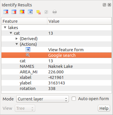
地物の選択とアクションの指定

When we click on the action, it brings up Firefox and navigates to the URL http://www.google.com/search?q=Tustumena. It is also possible to add further attribute fields to the action. Therefore, you can add a + to the end of the action text, select another field and click on [Insert Field]. In this example, there is just no other field available that would make sense to search for.

You can define multiple actions for a layer, and each will show up in the Identify Results dialog.

There are all kinds of uses for actions. For example, if you have a point layer containing locations of images or photos along with a file name, you could create an action to launch a viewer to display the image. You could also use actions to launch web-based reports for an attribute field or combination of fields, specifying them in the same way we did in our Google search example.

また、より複雑な例を作成できます。例えば、Python アクションを使用できます。

Usually, when we create an action to open a file with an external application, we can use absolute paths, or eventually relative paths. In the second case, the path is relative to the location of the external program executable file. But what about if we need to use relative paths, relative to the selected layer (a file-based one, like a shapefile or SpatiaLite)? The following code will do the trick:

command = "firefox";
imagerelpath = "images_test/test_image.jpg";
layer = qgis.utils.iface.activeLayer();
import os.path;
layerpath = layer.source() if layer.providerType() == 'ogr'
  else (qgis.core.QgsDataSourceURI(layer.source()).database()
  if layer.providerType() == 'spatialite' else None);
path = os.path.dirname(str(layerpath));
image = os.path.join(path,imagerelpath);
import subprocess;
subprocess.Popen( [command, image ] );

We just have to remember that the action is one of type Python and the command and imagerelpath variables must be changed to fit our needs.

But what about if the relative path needs to be relative to the (saved) project file? The code of the Python action would be:

command="firefox";
imagerelpath="images/test_image.jpg";
projectpath=qgis.core.QgsProject.instance().fileName();
import os.path; path=os.path.dirname(str(projectpath)) if projectpath != '' else None;
image=os.path.join(path, imagerelpath);
import subprocess;
subprocess.Popen( [command, image ] );

Another Python action example is the one that allows us to add new layers to the project. For instance, the following examples will add to the project respectively a vector and a raster. The names of the files to be added to the project and the names to be given to the layers are data driven (filename and layername are column names of the table of attributes of the vector where the action was created):

qgis.utils.iface.addVectorLayer('/yourpath/[% "filename" %].shp','[% "layername" %]',
  'ogr')

ラスタ(この例ではTIFイメージ)を追加するには、次のようになります:

qgis.utils.iface.addRasterLayer('/yourpath/[% "filename" %].tif','[% "layername" %]
')

結合メニュー¶

The Joins menu allows you to join a loaded attribute table to a loaded vector layer. After clicking , the Add vector join dialog appears. As key columns, you have to define a join layer you want to connect with the target vector layer. Then, you have to specify the join field that is common to both the join layer and the target layer. Now you can also specify a subset of fields from the joined layer based on the checkbox Choose which fields are joined. As a result of the join, all information from the join layer and the target layer are displayed in the attribute table of the target layer as joined information. If you specified a subset of fields only these fields are displayed in the attribute table of the target layer.

QGIS currently has support for joining non-spatial table formats supported by OGR (e.g., CSV, DBF and Excel), delimited text and the PostgreSQL provider (see figure_joins_1).

Figure Joins 1:

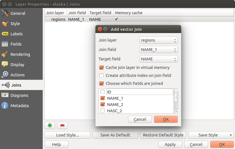
既存ベクタレイヤの属性テーブルを結合します

さらにベクタ結合ダイアログでは次のことができます:

• 結合レイヤをヴァーチャルメモリにキャッシュする

• 結合フィールドに属性インデックスを作成する

ダイアグラムメニュー¶

ダイアグラム メニューではベクタレイヤにグラフィックオーバーレイを行うことができます ( figure_diagrams_1 参照).

現状のダイアグラムのコア実装はパイチャート、テキストダイアグラムとヒストグラムが提供されています.

The menu is divided into four tabs: Appearance, Size, Postion and Options.

In the cases of the text diagram and pie chart, text values of different data columns are displayed one below the other with a circle or a box and dividers. In the Size tab, diagram size is based on a fixed size or on linear scaling according to a classification attribute. The placement of the diagrams, which is done in the Position tab, interacts with the new labeling, so position conflicts between diagrams and labels are detected and solved. In addition, chart positions can be fixed manually.

Figure Diagrams 1:

ダイアグラムメニューを表示したベクタプロパティダイアログ

We will demonstrate an example and overlay on the Alaska boundary layer a text diagram showing temperature data from a climate vector layer. Both vector layers are part of the QGIS sample dataset (see section サンプルデータ).

1. First, click on the ^{Load Vector} icon, browse to the QGIS sample dataset folder, and load the two vector shape layers alaska.shp and climate.shp.

2. 地図凡例にある climate layer をダブルクリックして レイヤプロパティ ダイアログを開いて下さい.

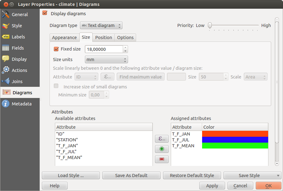
3. Click on the Diagrams menu, activate Display diagrams, and from the Diagram type combo box, select ‘Text diagram’.
4. In the Appearance tab, we choose a light blue as background color, and in the Size tab, we set a fixed size to 18 mm.
5. In the Position tab, placement could be set to ‘Around Point’.
6. In the diagram, we want to display the values of the three columns T_F_JAN, T_F_JUL and T_F_MEAN. First select T_F_JAN as Attributes and click the button, then T_F_JUL, and finally T_F_MEAN.

7. ここで [Apply] をクリックすると QGIS メインウィンドウにダイアグラムが表示されます.

8. You can adapt the chart size in the Size tab. Deactivate the Fixed size and set the size of the diagrams on the basis of an attribute with the [Find maximum value] button and the Size menu. If the diagrams appear too small on the screen, you can activate the Increase size of small diagrams checkbox and define the minimum size of the diagrams.
9. Change the attribute colors by double clicking on the color values in the Assigned attributes field. Figure_diagrams_2 gives an idea of the result.

10. 最後に**[OK]**をクリックします。

Figure Diagrams 2:

気温データのダイアグラムの地図オーバーレイ表示

Remember that in the Position tab, a Data defined position of the diagrams is possible. Here, you can use attributes to define the position of the diagram. You can also set a scale-dependent visibility in the Appearance tab.

The size and the attributes can also be an expression. Use the button to add an expression. See Expressions chapter for more information and example.

メタデータメニュー¶

The Metadata menu consists of Description, Attribution, MetadataURL and Properties sections.

In the Properties section, you get general information about the layer, including specifics about the type and location, number of features, feature type, and editing capabilities. The Extents table provides you with layer extent information and the Layer Spatial Reference System, which is information about the CRS of the layer. This is a quick way to get information about the layer.

Additionally, you can add or edit a title and abstract for the layer in the Description section. It’s also possible to define a Keyword list here. These keyword lists can be used in a metadata catalogue. If you want to use a title from an XML metadata file, you have to fill in a link in the DataUrl field. Use Attribution to get attribute data from an XML metadata catalogue. In MetadataUrl, you can define the general path to the XML metadata catalogue. This information will be saved in the QGIS project file for subsequent sessions and will be used for QGIS server.

Figure Metadata 1:

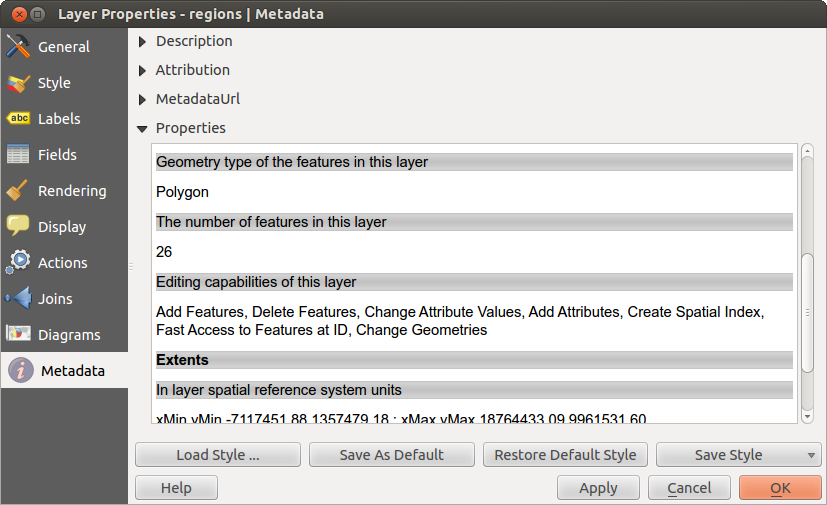
ベクタプロパティダイアログのメタデータメニュー